Problems
- Decaying learning rates provide googd compromise between escaping poor local minima and convergence
- Many of the convergence issues arise because we force the same learning rate on all parameters
- Try to releasing the requirement that a fixed step size is used across all dimensions
- To be clear, backpropagation is a way to compute derivative, not a algorithm
- The below is NOT grident desent algorithm
Better convergence strategy
Derivative-inspired algorithms
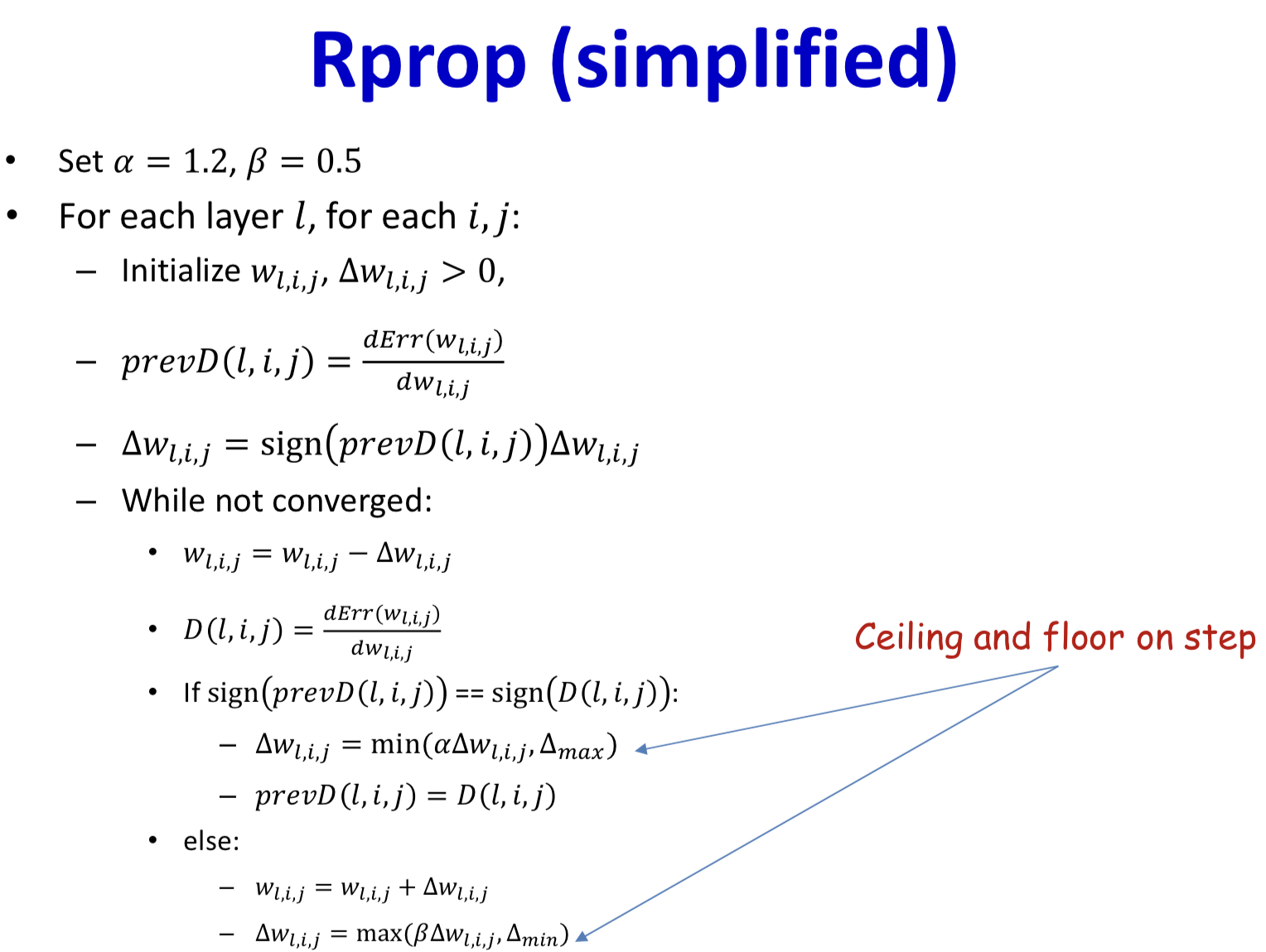
RProp
- Resilient propagation
- Simple first-order algorithm, to be followed independently for each component
- Steps in different directions are not coupled
- At each time
- If the derivative at the current location recommends continuing in the same direction as before (i.e. has not changed sign from earlier):
- Increase the step( > 1), and continue in the same direction
- If the derivative has changed sign (i.e. we’ve overshot a minimum)
- Reduce the step() and reverse direction
- If the derivative at the current location recommends continuing in the same direction as before (i.e. has not changed sign from earlier):
- Features
- It is frequently much more efficient than gradient descent
- No convexity assumption
QuickProp
- Newton updates
Quickprop employs the Newton updates with two modifications
It treats each dimension independently
- It approximates the second derivative through finite differences
- Features
- Employs Newton updates with empirically derived derivatives
- Prone to some instability for non-convex objective functions
- But is still one of the fastest training algorithms for many problems
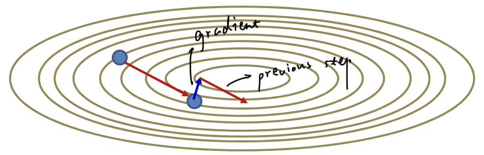
Momentum methods
- Insight
- In the direction that converges, it keeps pointing in the same direction
- Need keep track of oscillations
- Emphasize steps in directions that converge smoothly
- In the direction that overshoots, it steps back and forth
- Shrink steps in directions that bounce around
- In the direction that converges, it keeps pointing in the same direction
- Maintain a running average of all past steps
- Get longer in directions where gradient stays in the same sign
- Become shorter in directions where the sign keep flipping
- Update with the running average, rather than the current gradient
- Emphasize directions of steady improvement are demonstrably superior to other methods
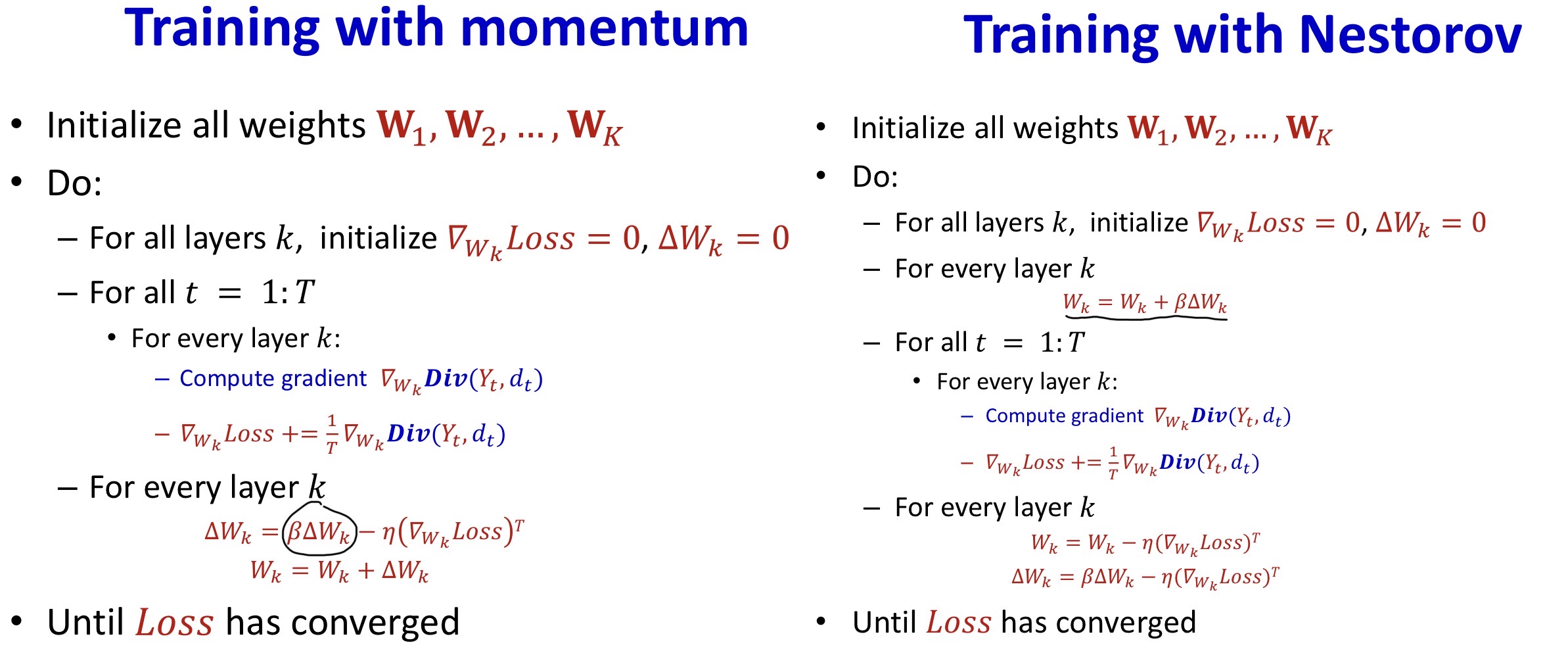
- Momentum Update
- First computes the gradient step at the current location:
- Then adds in the scaled previous step:
Nestorov’s Accelerated Gradient
- Change the order of operations
- First extend the previous step:
- Then compute the gradient step at the resultant position:
- Add the two to obtain the final step
- Converges much faster than momentum
Summary
- Try the step size for all dimension is bad
- Treat each dimension independently
- Try to normalize curvature in all directions
- Second order methods, e.g. Newton's method
- Too expensive: require inversion of a giant Hessian
- Treat each dimension independently
- RProp / QucikProp
- Works, but ignores dependence between dimensions
- Can still be too slow
- Momentum methods which emphasize directions of steady improvement are demonstrably superior to other methods
Incremental updates
- Batch gradient descent
- Try to simultaneously adjust the function at all training points
- We must process all training points before making a single adjustment
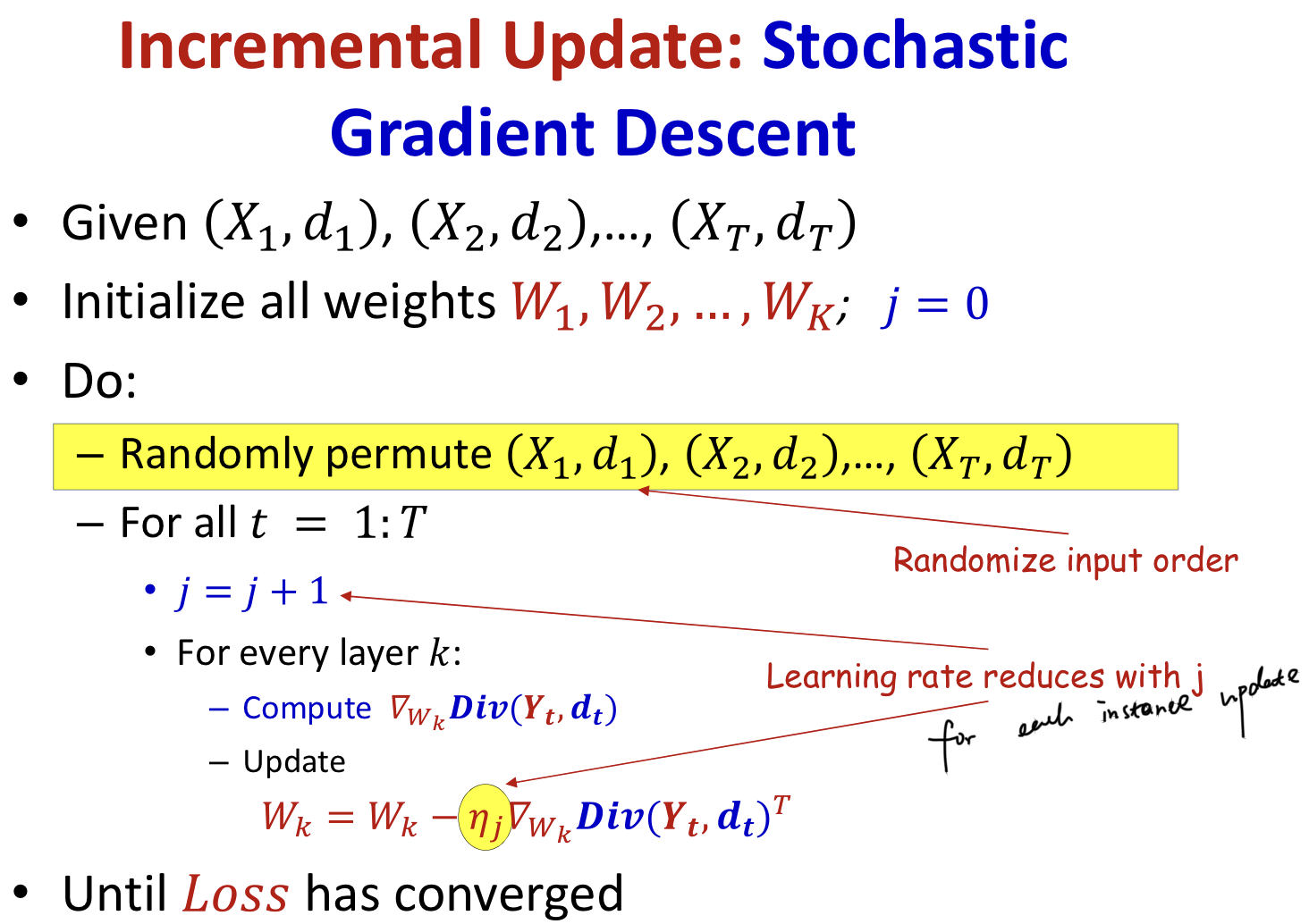
- Stochastic gradient descent
- Adjust the function at one training point at a time
- A single pass through the entire training data is called an “epoch”
- An epoch over a training set with samples result in updates of parameters
- We must go through them randomly to get more convergent behavior
- Otherwise we may get cyclic behavior (hard to converge)
- Learning rate
- Correcting the function for individual instances will lead to never-ending, non-convergent updates (correct one, and miss the other)
- The learning will continuously “chase” the latest sample
- Correction for individual instances with the eventual miniscule learning rates will not modify the function
Drewbacks
- Batch / Stochastic gradient descent is an unbiased estimate of the expected loss
- But the variance of the empirical risk in batch gradient is {% math_inline %}\frac{1}{N}{% endmath_inline %} times compared to stochastic gradient descent
- Like using {% math_inline %}\frac{1}{N}\sum{X}{% endmath_inline %} and {% math_inline %}X_i{% endmath_inline %} to estimate {% math_inline %}\bar{X}{% endmath_inline %}
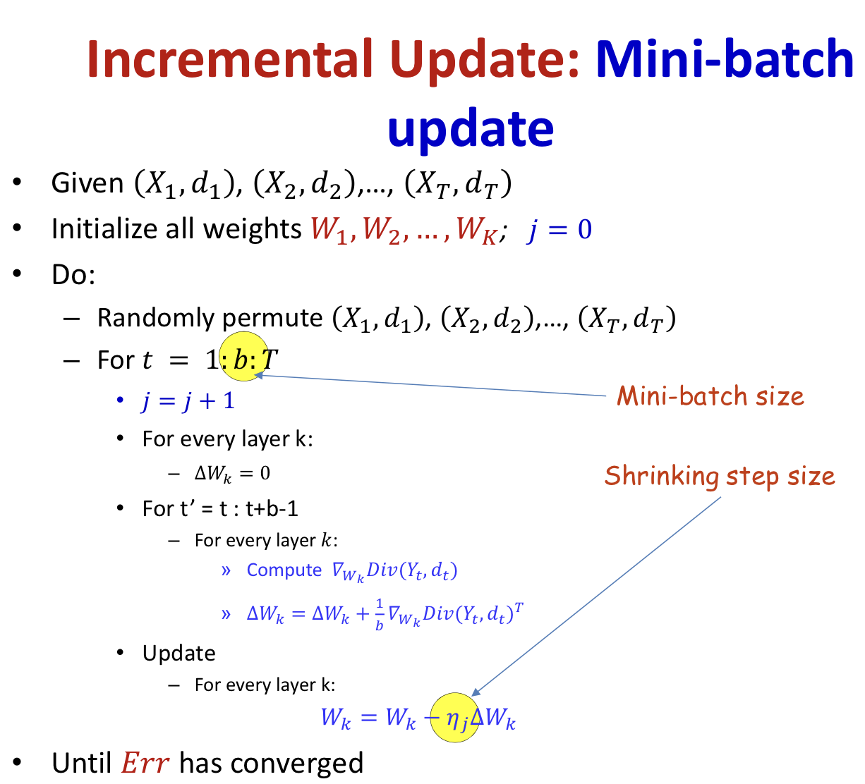
Mini-batch gradient descent
- Adjust the function at a small, randomly chosen subset of points
- Also an unbiased estimate of the expected error, and the variance is relatively small compared to SGD
- The mini-batch size is a hyper parameter to be optimized
- Convergence depends on learning rate
- Simple technique: fix learning rate until the error plateaus, then reduce learning rate by a fixed factor (e.g. 10)
- Advanced methods: Adaptive updates, where the learning rate is itself determined as part of the estimation