Modelling Series

• In many situations one must consider a series of inputs to produce an output

  • Outputs too may be a series

• Finite response model

  • Can use convolutional neural net applied to series data (slide)

    • Also called a Time-Delay neural network

  • Something that happens today only affects the output of the system for days into the future

    • $Y_{t}=f\left(X_{t}, X_{t-1}, \ldots, X_{t-N}\right)$

• Infinite response systems

  • Systems often have long-term dependencies

  • What happens today can continue to affect the output forever

    • $Y_{t}=f\left(X_{t}, X_{t-1}, \ldots, X_{t-\infty}\right)$

Infinite response systems

• A one-tap NARX network

  • 「nonlinear autoregressive network with exogenous inputs」
  • $Y_t = f(X_t,Y_{t-1})$
  • An input at t=0 affects outputs forever
  • 

• An explicit memory variable whose job it is to remember

  • $\begin{array}{c} m_{t}=r\left(y_{t-1}, h_{t-1}^{\prime}, m_{t-1}\right) \\\\ h_{t}=f\left(x_{t}, m_{t}\right) \\\\ y_{t}=g\left(h_{t}\right) \end{array}$

  • 

• Jordan Network

  • Memory unit simply retains a running average of past outputs
  • Memory has fixed structure; does not “learn” to remember

• Elman Networks

  • Separate memory state from output
  • Only the weight from the memory unit to the hidden unit is learned
    • But during training no gradient is backpropagated over the “1” link (Just cloned state)

• Problem

  • “Simple” (or partially recurrent) because during learning current error does not actually propagate to the past

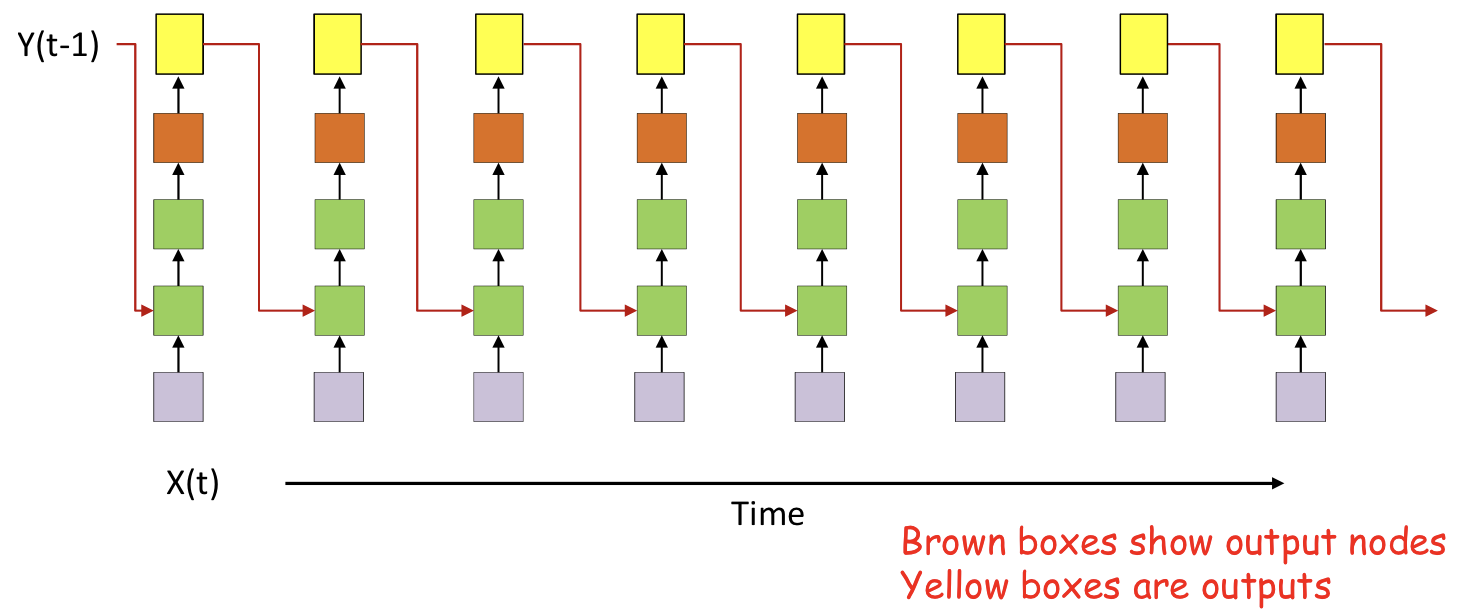
State-space model

$\begin{array}{c} h_{t}=f\left(x_{t}, h_{t-1}\right) \\\\ y_{t}=g\left(h_{t}\right) \end{array}$

• $h_t$ is the state of the network
  • Model directly embeds the memory in the state
  • State summarizes information about the entire past
• Recurrent neural network¹

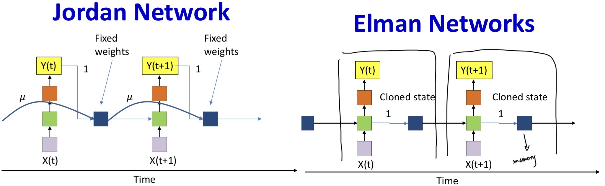
Variants

• All columns are identical

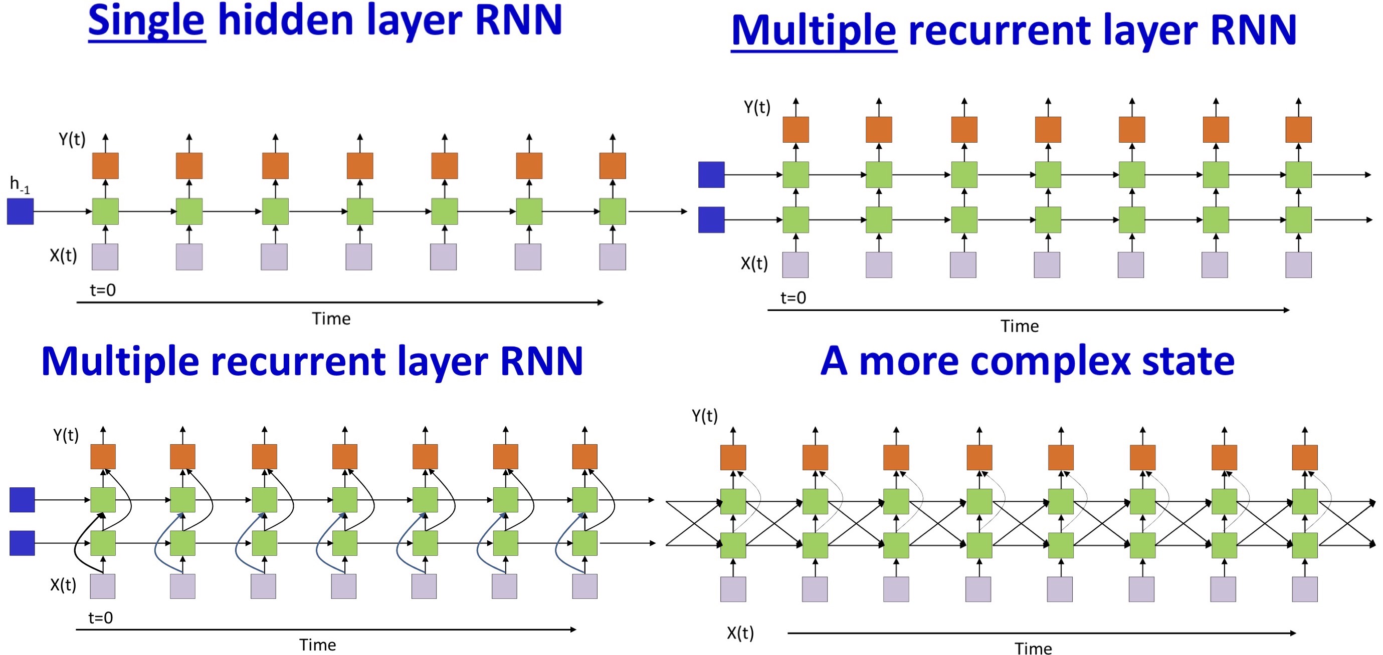
• The simplest structures are most popular

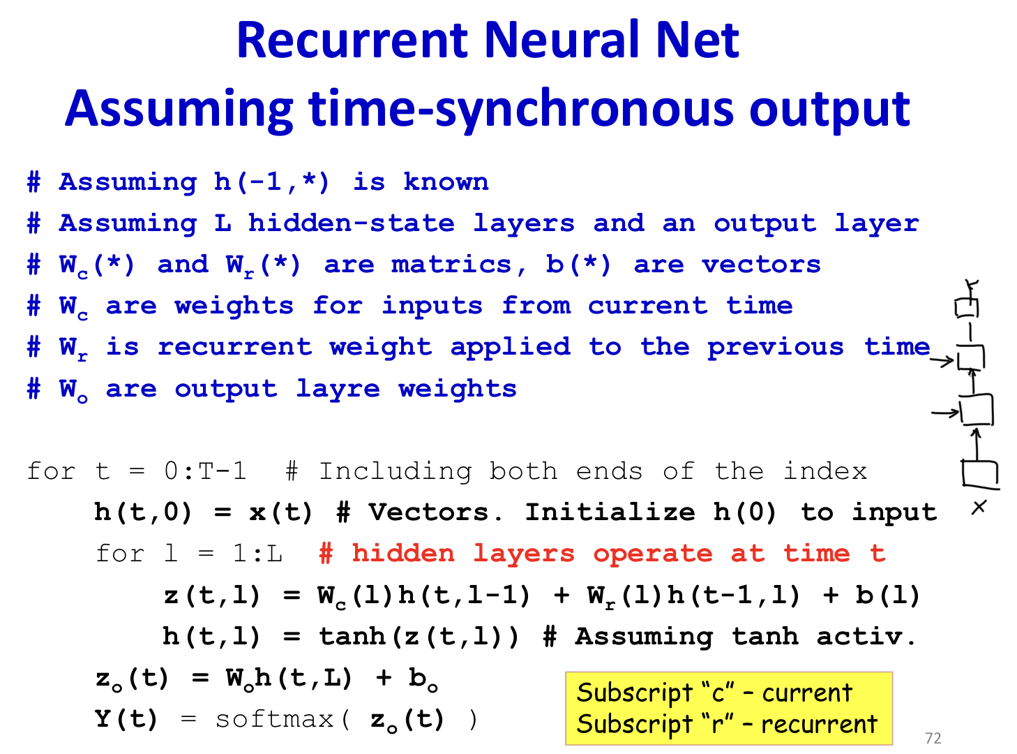
Recurrent neural network

Forward pass

Backward pass

• BPTT
  • Back Propagation Through Time
  • Defining a divergence between the actual and desired output sequences
  • Backpropagating gradients over the entire chain of recursion
    • Backpropagation through time
  • Pooling gradients with respect to individual parameters over time

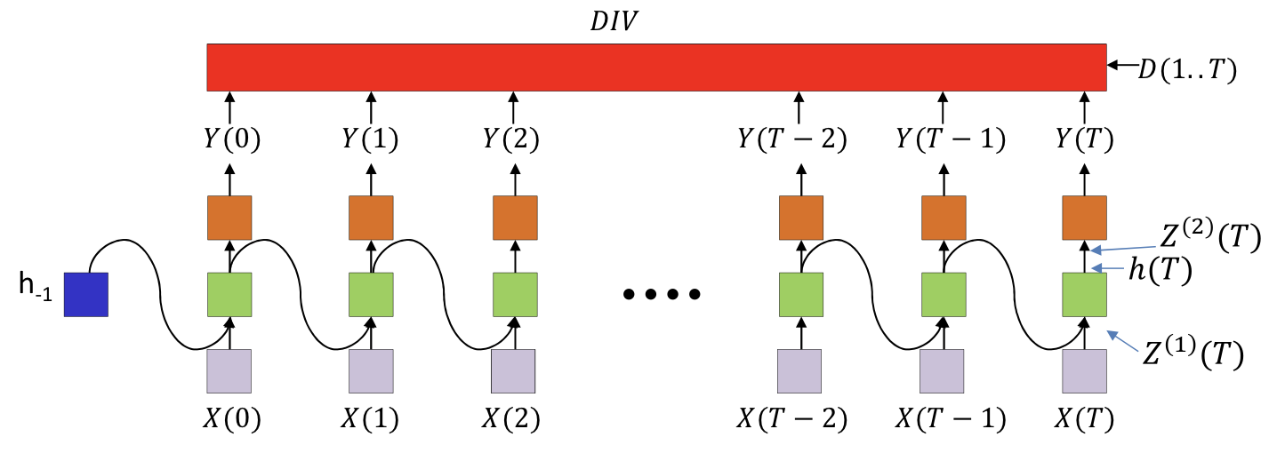
Notion

• The divergence computed is between the sequence of outputs by the network and the desired sequence of outputs
  • DIV is a scalar function of a ..series.. of vectors
  • This is not just the sum of the divergences at individual times
• $Y(t)$ is the output at time $t$
  • $Y_i(t)$ is the ith output
• $Z^{(2)}(t)$ is the pre-activation value of the neurons at the output layer at time $t$
• $h(t)$ is the output of the hidden layer at time $t$

BPTT

• $Y(t)$ is a column vector
• $DIV$ is a scalar
• $\frac{d Div}{d Y(t)}$ is a row vector

Derivative at time $T$

1. Compute $\frac{d DIV}{d Y_i(T)}$ for all $i$

   • In general we will be required to compute $\frac{d DIV}{d Y_i(t)}$ for all $i$ and $t$ as we will see

     • This can be a source of significant difficulty in many scenarios

   • Special case, when the overall divergence is a simple sum of local divergences at each time

     • $\frac{d D I V}{d Y_{i}(t)}=\frac{d D i v(t)}{d Y_{i}(t)}$

2. Compute $\nabla_{Z^{(2)}(T)}{D I V}$

   • $\nabla_{Z^{(2)}(T)}{D I V}=\nabla_{Y(T)} D I V \nabla_{Z^{(2)}(T)} Y(T)$

   • For scalar output activation

     • $\frac{d D I V}{d Z_{i}^{(2)}(T)}=\frac{d D I V}{d Y_{i}(T)} \frac{d Y_{i}(T)}{d Z_{i}^{(2)}(T)}$

   • For vector output activation

     • $\frac{d D I V}{d Z_{i}^{(2)}(T)}=\sum_{i} \frac{d D I V}{d Y_{j}(T)} \frac{d Y_{j}(T)}{d Z_{i}^{(2)}(T)}$

3. Compute $\nabla_{h_(T)}{D I V}$

   • $W^{(2)} h(T) = Z^{(2)}(T)$

   • $\frac{d D I V}{d h_{i}(T)}=\sum_{j} \frac{d D I V}{d Z_{j}^{(2)}(T)} \frac{d Z_{j}^{(2)}(T)}{d h_{i}(T)}=\sum_{j} w_{i j}^{(2)} \frac{d D I V}{d Z_{j}^{(2)}(T)}$

   • $\nabla_{h(T)} D I V=\nabla_{Z^{(2)}(T)} D I V W^{(2)}$

4. Compute $\nabla_{W^{(2)}}{D I V}$

   • $\frac{d D I V}{d w_{i j}^{(2)}}=\frac{d D I V}{d Z_{j}^{(2)}(T)} h_{i}(T)$

   • $\nabla_{W^{(2)}} D I V=h(T) \nabla_{Z^{(2)}(T)} D I V$

5. Compute $\nabla_{Z^{(1)}(T)}{D I V}$

   • $\frac{d D I V}{d Z_{i}^{(1)}(T)}=\frac{d D I V}{d h_{i}(T)} \frac{d h_{i}(T)}{d Z_{i}^{(1)}(T)}$

   • $\nabla_{Z^{(1)}(T)} D I V=\nabla_{h(T)} D I V \nabla_{Z^{(1)}(T)} h(T)$

6. Compute $\nabla_{W^{(1)}}{D I V}$

   • $W^{(1)} X(T) + W^{(11)} h(T-1)= Z^{(1)}(T)$

   • $\frac{d D I V}{d w_{i j}^{(1)}}=\frac{d D I V}{d Z_{j}^{(1)}(T)} X_{i}(T)$

   • $\nabla_{W^{(1)}} D I V=X(T) \nabla_{Z^{(1)}(T)} D I V$

7. Compute $\nabla_{W^{(11)}}{D I V}$

   • $\frac{d D I V}{d w_{i i}^{(11)}}=\frac{d D I V}{d Z_{i}^{(1)}(T)} h_{i}(T-1)$

   • $\nabla_{W}^{(11)} D I V=h(T-1) \nabla_{Z^{(1)}(T)} D I V$

Derivative at time $T-1$

1. Compute $\nabla_{Z^{(2)}(T-1)}{D I V}$

   • $\nabla_{Z^{(2)}(T-1)}{D I V}=\nabla_{Y(T-1)} D I V \nabla_{Z^{(2)}(T-1)} Y(T-1)$

   • For scalar output activation

     • $\frac{d D I V}{d Z_{i}^{(2)}(T-1)}=\frac{d D I V}{d Y_{i}(T-1)} \frac{d Y_{i}(T-1)}{d Z_{i}^{(2)}(T-1)}$

   • For vector output activation

     • $\frac{d D I V}{d Z_{i}^{(2)}(T-1)}=\sum_{j} \frac{d D I V}{d Y_{j}(T-1)} \frac{d Y_{j}(T-1)}{d Z_{i}^{(2)}(T-1)}$

2. Compute $\nabla_{h_(T-1)}{D I V}$

   • $\frac{d D I V}{d h_{i}(T-1)}=\sum_{j} w_{i j}^{(2)} \frac{d D I V}{d Z_{j}^{(2)}(T-1)}+\sum_{j} w_{i j}^{(11)} \frac{d D I V}{d Z_{j}^{(1)}(T)}$

   • $\nabla_{h(T-1)} D I V=\nabla_{Z^{(2)}(T-1)} D I V W^{(2)}+\nabla_{Z^{(1)}(T)} D I V W^{(11)}$

3. Compute $\nabla_{W^{(2)}}{D I V}$

   • $\frac{d D I V}{d w_{i j}^{(2)}}+=\frac{d D I V}{d Z_{j}^{(2)}(T-1)} h_{i}(T-1)$

   • $\nabla_{W^{(2)}} D I V+=h(T-1) \nabla_{Z^{(2)}(T-1)} D I V$

4. Compute $\nabla_{Z^{(1)}(T-1)}{D I V}$

   • $\frac{d D I V}{d Z_{i}^{(1)}(T-1)}=\frac{d D I V}{d h_{i}(T-1)} \frac{d h_{i}(T-1)}{d Z_{i}^{(1)}(T-1)}$

   • $\nabla_{Z^{(1)}(T-1)} D I V=\nabla_{h(T-1)} D I V \nabla_{Z^{(1)}(T-1)} h(T-1)$

5. Compute $\nabla_{W^{(1)}}{D I V}$

   • $\frac{d D I V}{d w_{i j}^{(1)}}+=\frac{d D I V}{d Z_{j}^{(1)}(T-1)} X_{i}(T-1)$

   • $\nabla_{W^{(1)}} D I V+=X(T-1) \nabla_{Z^{(1)}(T-1)} D I V$

6. Compute $\nabla_{W^{(11)}}{D I V}$

   • $\frac{d D I V}{d w_{i j}^{(11)}}+=\frac{d D I V}{d Z_{j}^{(1)}(T-1)} h_{i}(T-2)$

     • {% math %} \nabla{W^{(11)}} D I V+=h(T-2) \nabla{Z^{(1)}(T-1)} D I V {% endmath %}

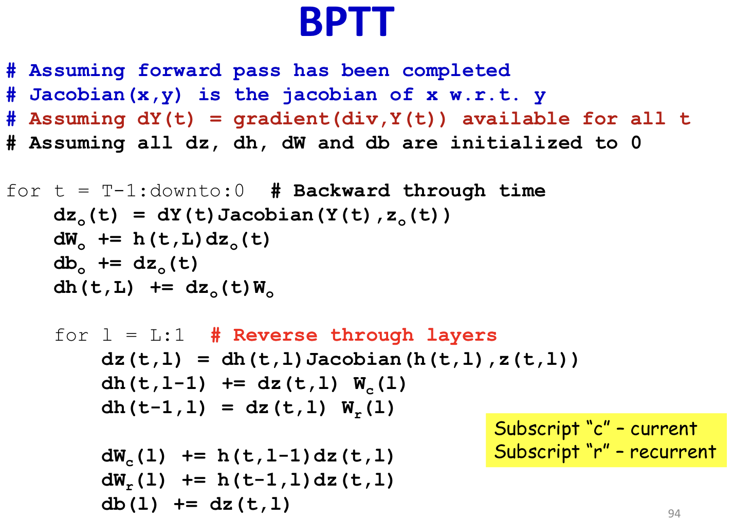
Back Propagation Through Time

$\frac{d D I V}{d h_{i}(-1)}=\sum_{i} w_{i j}^{(11)} \frac{d D I V}{d Z_{j}^{(1)}(0)}$

$\frac{d D I V}{d h_{i}^{(k)}(t)}=\sum_{j} w_{i, j}^{(k+1)} \frac{d D I V}{d Z_{j}^{(k+1)}(t)}+\sum_{j} w_{i, j}^{(k, k)} \frac{d D I V}{d Z_{j}^{(k)}(t+1)}$

$\frac{d D I V}{d Z_{i}^{(k)}(t)}=\frac{d D I V}{d h_{i}^{(k)}(t)} f_{k}^{\prime}\left(Z_{i}^{(k)}(t)\right)$

$\frac{d D I V}{d w_{i j}^{(1)}}=\sum_{t} \frac{d D I V}{d Z_{j}^{(1)}(t)} X_{i}(t)$

$\frac{d D I V}{d w_{i j}^{(11)}}=\sum_{t} \frac{d D I V}{d Z_{j}^{(1)}(t)} h_{i}(t-1)$

Algorithm

Bidirectional RNN

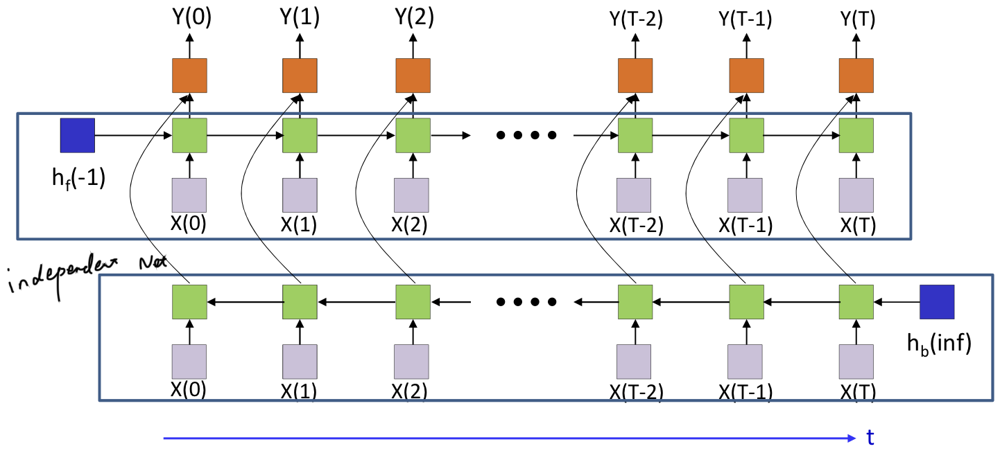
• Two independent RNN
• Clearly, this is not an online process and requires the entire input data
• It is easy to learning two RNN independently
  • Forward pass: Compute both forward and backward networks and final output
  • Backpropagation
    • A basic backprop routine that we will call
    • Two calls to the routine within a higher-level wrapper

¹:The Unreasonable Effectiveness of Recurrent Neural Networks