Sequence to sequence

• Sequence goes in, sequence comes out
• No notion of “time synchrony” between input and output
  • May even nots maintain order of symbols (from one language to another)

With order synchrony

• The input and output sequences happen in the same order
  • Although they may be time asynchronous
  • E.g. Speech recognition
    • The input speech corresponds to the phoneme sequence output
• Question
  • How do we know when to output symbols
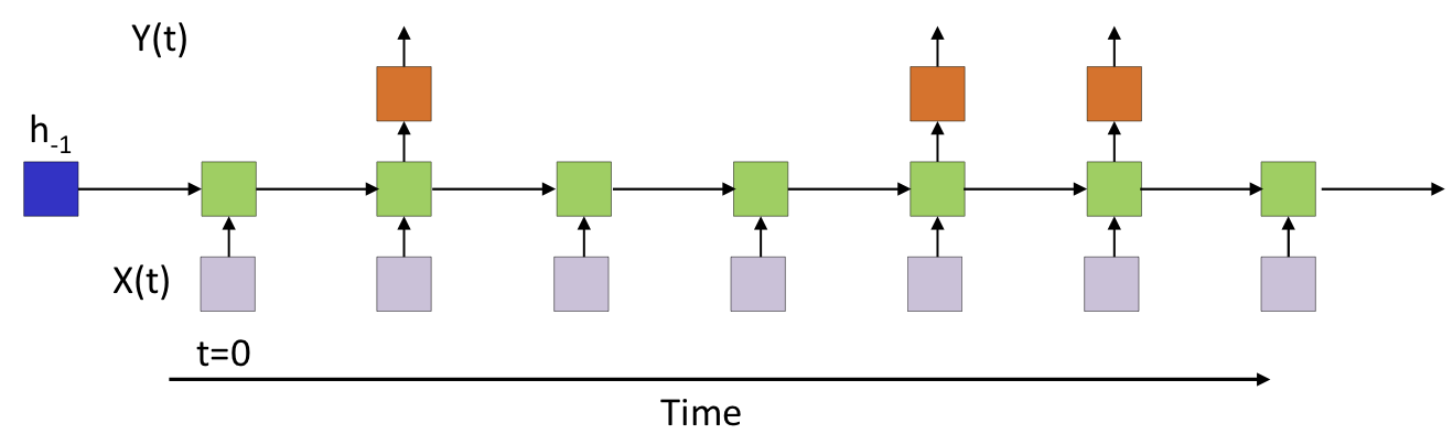
  • In fact, the network produces outputs at every time
  • Which of these are the real outputs?

Option 1

• Simply select the most probable symbol at each time
• Merge adjacent repeated symbols, and place the actual emission of the symbol in the final instant
• Problem
  • Cannot distinguish between an extended symbol and repetitions of the symbol
  • Resulting sequence may be meaningless

Option 2

• Impose external constraints on what sequences are allowed
  • E.g. only allow sequences corresponding to dictionary words

Decoding

• The process of obtaining an output from the network

• Time-synchronous & order-synchronous sequence

  • aaabbbbbbccc => abc (probility 0.5)
    aabbbbbbbccc => abc (probility 0.001)
    cccddddddeee => cde (probility 0.4)
    cccddddeeeee => cde (probility 0.4)
    

  • So abc is the most likely time-synchronous output sequence
  • But cde is the the most likely order-synchronous sequence

• Option 2 is in fact a suboptimal decode that actually finds the most likely time-synchronous output sequence

• The “merging” heuristics do not guarantee optimal order-synchronous sequences

No timing information provided

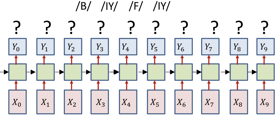
• Only the sequence of output symbols is provided for the training data
  • But no indication of which one occurs where

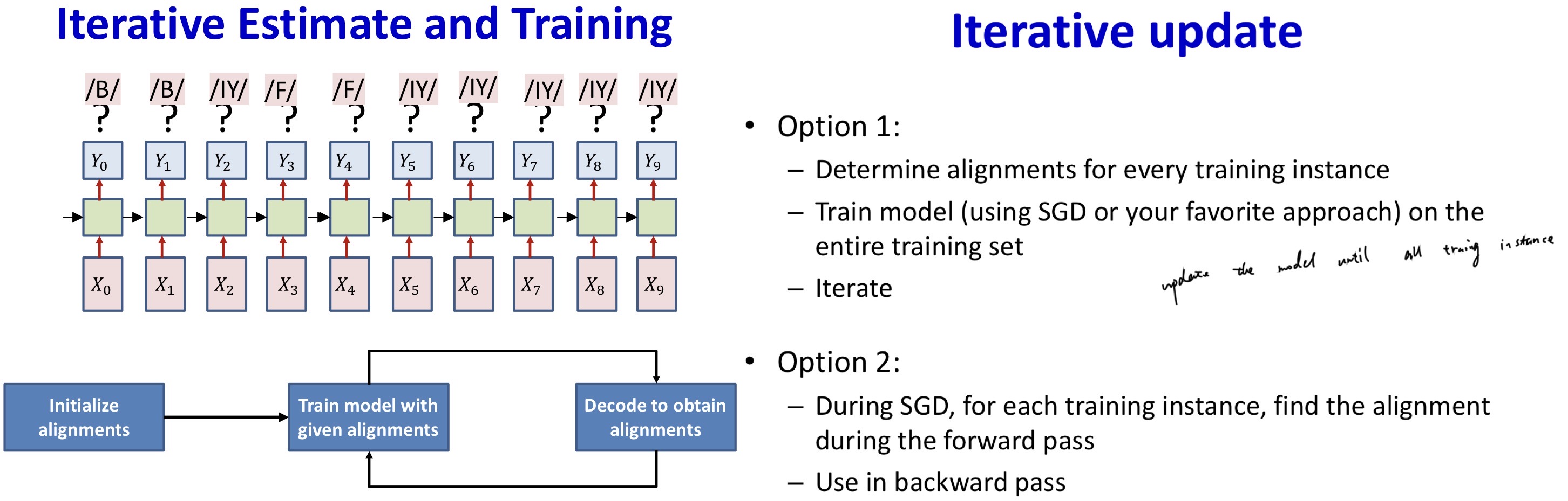
Guess the alignment

• Initialize
  • Assign an initial alignment
  • Either randomly, based on some heuristic, or any other rationale
• Iterate
  • Train the network using the current alignment
  • Reestimate the alignment for each training instance

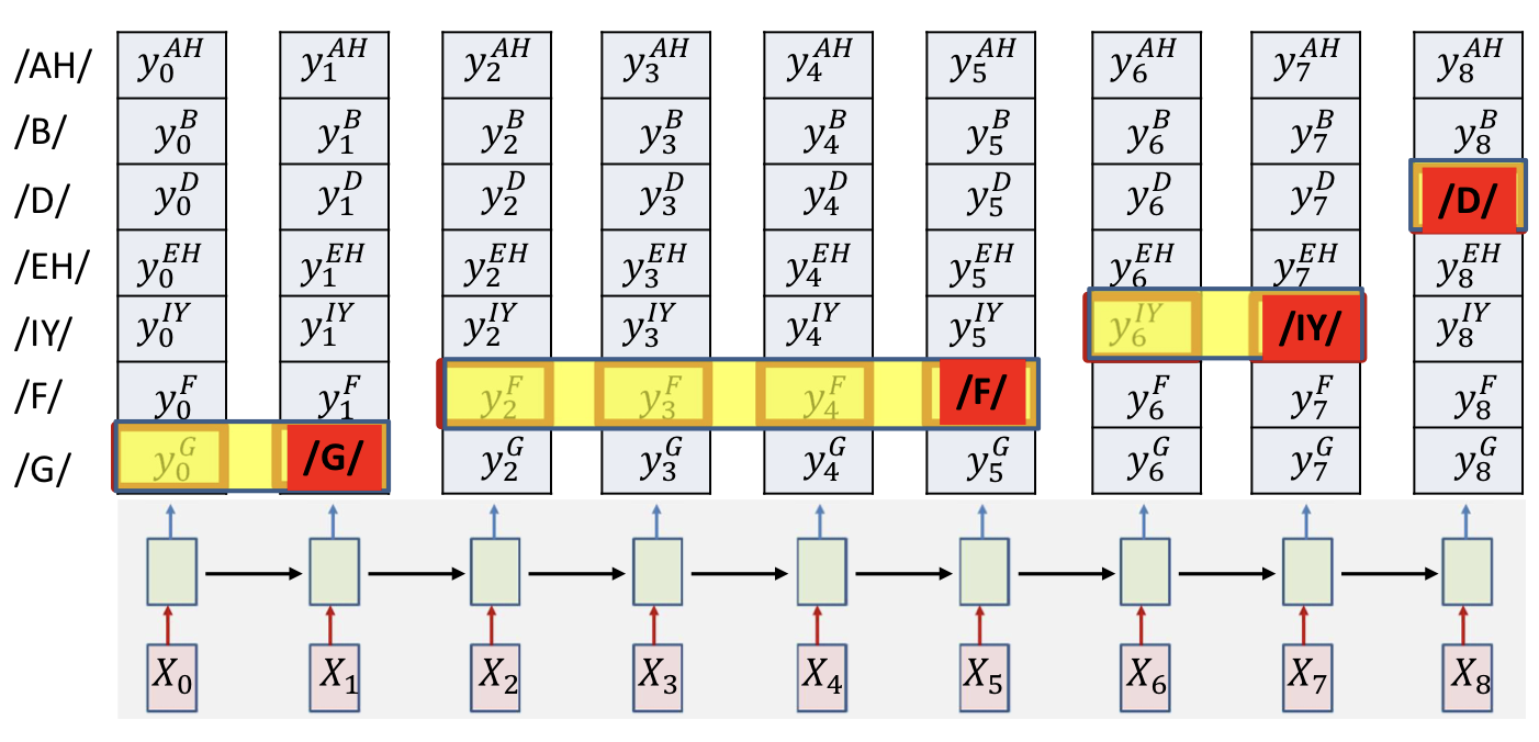
Constraining the alignment

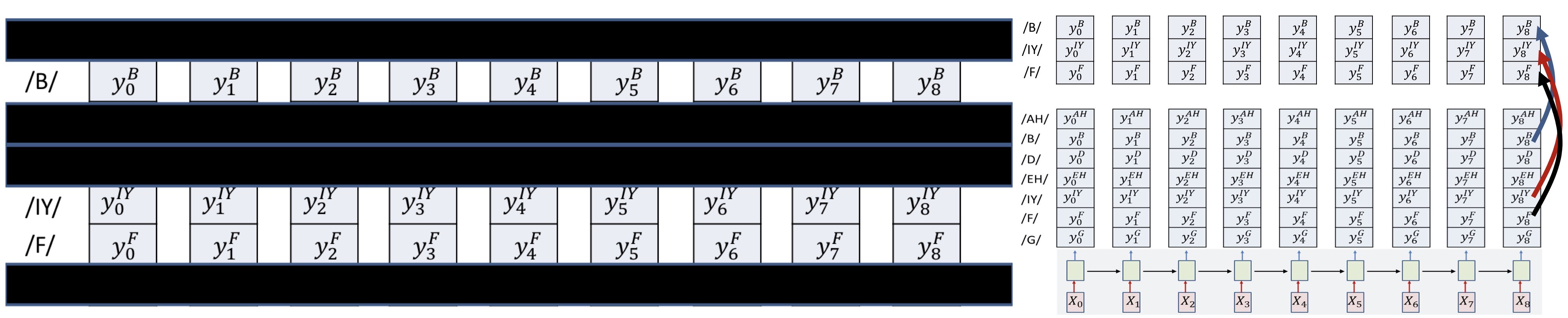
• Try 1
  • Block out all rows that do not include symbols from the target sequence
  • E.g. Block out rows that are not /B/ /IY/ or /F/
• Only decode on reduced grid
  • We are now assured that only the appropriate symbols will be hypothesized
• But this still doesn’t assure that the decode sequence correctly expands the target symbol sequence
  • Order variance
• Try 2
  • Explicitly arrange the constructed table
  • Arrange the constructed table so that from top to bottom it has the exact sequence of symbols required
    • If a symbol occurs multiple times, we repeat the row in the appropriate location

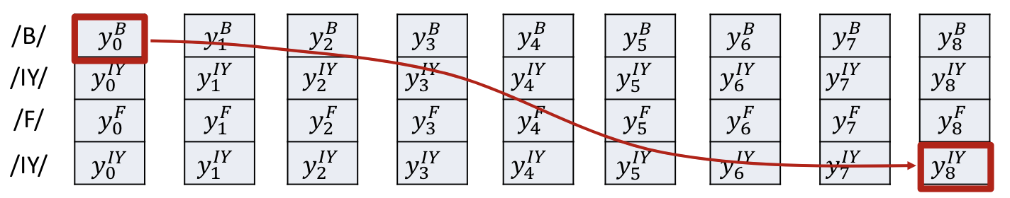
• Constrain that the first symbol in the decode must be the top left block

  • The last symbol must be the bottom right
  • The rest of the symbols must follow a sequence that monotonically travels down from top left to bottom right
  • This guarantees that the sequence is an expansion of the target sequence

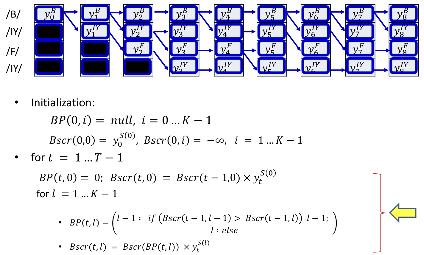
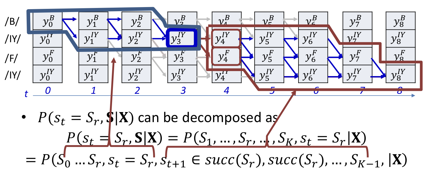
• Compose a graph such that every path in the graph from source to sink represents a valid alignment

  • The “score” of a path is the product of the probabilities of all nodes along the path
  • Find the most probable path from source to sink using any dynamic programming algorithm (viterbi algorithm)

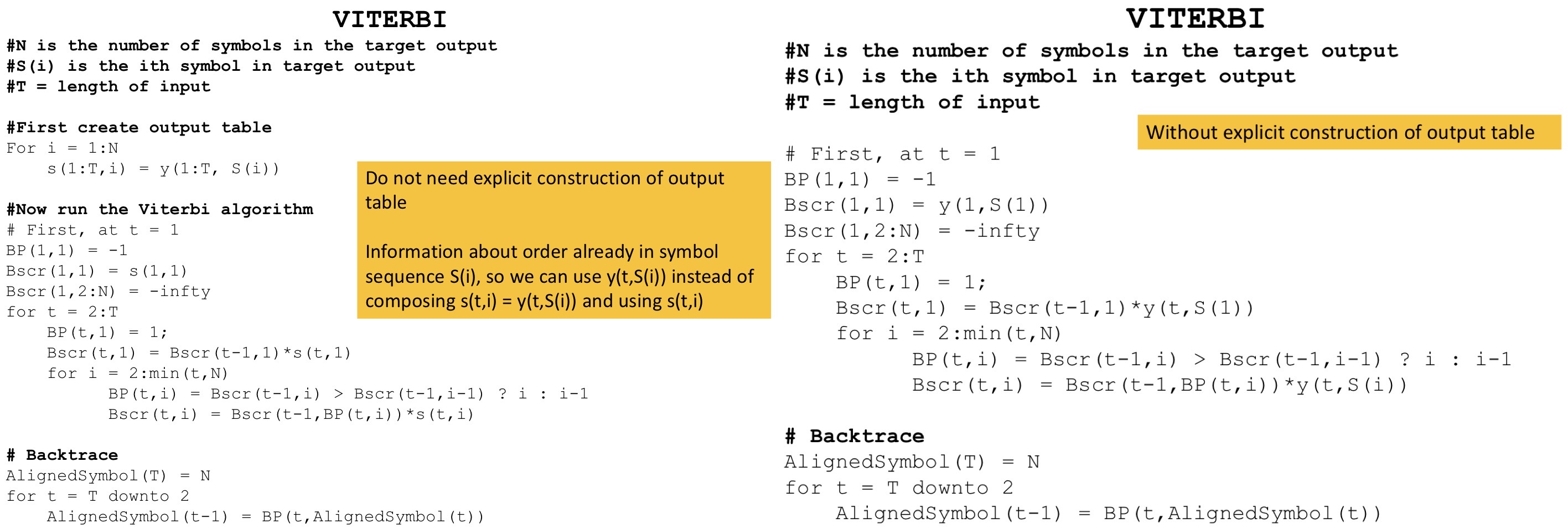
Viterbi algorithm

• Main idea
  • The best path to any node must be an extension of the best path to one of its parent nodes

• Dynamically track the best path (and the score of the best path) from the source node to every node in the graph

  • At each node, keep track of
    • The best incoming parent edge (BP)
    • The score of the best path from the source to the node through this best parent edge (Bscr)

• Process

  • 
• Algorithm
  • 

Gradients

$D I V=\sum_{t} X e n t\left(Y_{t}, s y m b o l_{t}^{b e s t p a t h}\right)=-\sum_{t} \log Y\left(t, s y m b o l_{t}^{b e s t p a t h}\right)$

• The gradient w.r.t the -th output vector $Y_t$ $\nabla_{Y_{t}} D I V=[0 \quad 0 \cdot \cdot \cdot \frac{-1}{Y(t, s y m b o l_{t}^{b e s t p a t h})} \quad 0 \cdot \cdot \cdot 0]$

• Problem

  • Approach heavily dependent on initial alignment
  • Prone to poor local optima
    • Because we commit to the single “best” estimated alignment
    • This can be way off, particularly in early iterations, or if the model is poorly initialized

• Alternate view

  • There is a probability distribution over alignments of the target Symbol sequence (to the input)
  • Selecting a single alignment is the same as drawing a single sample from it

• Instead of only selecting the most likely alignment, use the statistical expectation over all possible alignments

  • $D I V=E\left[-\sum_{t} \log Y\left(t, s_{t}\right)\right]$

  • Use the entire distribution of alignments

  • This will mitigate the issue of suboptimal selection of alignment

• Using the linearity of expectation

  • $D I V=-\sum_{t} E\left[\log Y\left(t, s_{t}\right)\right]$

  • $D I V=-\sum_{t} \sum_{S \in S_{1} \ldots S_{K}} P\left(s_{t}=S | \mathbf{S}, \mathbf{X}\right) \log Y\left(t, s_{t}=S\right)$

A posteriori probabilities of symbols

• $P(s_{t}=S | \mathbf{S}, \mathbf{X})$ is the probability of seeing the specific symbol $s$ at time $t$, given that the symbol sequence is an expansion of $S = s_0,...,S_{K-1}$ and given the input sequence $X = X_o,...,X_{N-1}$

  • $P\left(s_{t}=S_{r} | \mathbf{S}, \mathbf{X}\right) \propto P\left(s_{t}=S_{r}, \mathbf{S} | \mathbf{X}\right)$
• $P\left(s_{t}=S_{r}, \mathbf{S} | \mathbf{X}\right)$ is the total probability of all valid paths in the graph for target sequence $S$ that go through the symbol $S_r$ (the $r^{th}$ symbol in the sequence $S_0,...,S_{K-1}$ ) at time

• For a recurrent network without feedback from the output we can make the conditional independence assumption

$P\left(s_{t}=S_{r}, \mathbf{S} | \mathbf{X}\right)=P\left(S_{0} \ldots S_{r}, s_{t}=S_{r} | \mathbf{X}\right) P\left(s_{t+1} \in \operatorname{succ}\left(S_{r}\right), \operatorname{succ}\left(S_{r}\right), \ldots, S_{K-1} | \mathbf{X}\right)$

• We will call the first term the forward probability $\alpha(t,r)$
• We will call the second term the backward probability $\beta(t,r)$

Forward algorithm

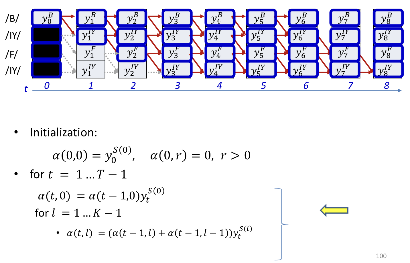
• In practice the recursion will gererally underflow

$\alpha(t, l)=(\alpha(t-1, l)+\alpha(t-1, l-1)) y_{t}^{S(l)}$

• Instead we can do it in the log domain

$\log \alpha(t, l)=\log \left(e^{\log \alpha(t-1, l)}+e^{\log \alpha(t-1, l-1)}\right)+\log y_{t}^{S(l)}$

Backward algorithm

$\beta(t, r)=P\left(s_{t+1} \in \operatorname{succ}\left(S_{r}\right), \operatorname{succ}\left(S_{r}\right), \ldots, S_{K-1} | \mathbf{X}\right)$

The joint probability

$P\left(s_{t}=S_{r}, \mathbf{S} | \mathbf{X}\right)=\alpha(t, r) \beta(t, r)$

• Need to be normalized, get posterior probability

$\gamma(t,r) = P\left(s_{t}=S_{r} | \mathbf{S}, \mathbf{X}\right)=\frac{P\left(s_{t}=S_{r}, \mathbf{S} | \mathbf{X}\right)}{\sum_{S_{r}^{\prime}} P\left(s_{t}=S_{r}^{\prime}, \mathbf{S} | \mathbf{X}\right)}=\frac{\alpha(t, r) \beta(t, r)}{\sum_{r^{\prime}} \alpha\left(t, r^{\prime}\right) \beta\left(t, r^{\prime}\right)}$

• We can also write this using the modified beta formula as (you will see this in papers)

$\gamma(t, r)=\frac{\frac{1}{y_{t}^{S(r)}} \alpha(t, r) \hat{\beta}(t, r)}{\sum_{r^{\prime}} \frac{1}{y_{t}^{S(r)}} \alpha(t, r) \hat{\beta}(t, r)}$

The expected divergence

$D I V=-\sum_{t} \sum_{s \in S_{0} \ldots S_{K-1}} P\left(s_{t}=s | \mathbf{S}, \mathbf{X}\right) \log Y\left(t, s_{t}=s\right)$

$D I V=-\sum_{t} \sum_{r} \gamma(t, r) \log y_{t}^{S(r)}$

• The derivative of the divergence w.r.t the output $Y_t$ of the net at any time

$\nabla_{Y_{t}} D I V=\left[\begin{array}{llll} \frac{d D I V}{d y_{t}^{S_{0}}} & \frac{d D I V}{d y_{t}^{S_{1}}} & \cdots & \frac{d D I V}{d y_{t}^{S_{L-1}}} \end{array}\right]$

• Compare to Viterbi algorithm, components will be non-zero only for symbols that occur in the training instance

• Compute derivative

$\frac{d D I V}{d y_{t}^{l}}=-\sum_{r: S(r)=l} \frac{d}{d y_{t}^{S(r)}} \gamma(t, r) \log y_{t}^{S(r)}$

$\frac{d}{d y_{t}^{S(r)}} \gamma(t, r) \log y_{t}^{S(r)}=\frac{\gamma(t, r)}{y_{t}^{S(r)}}+\frac{d \gamma(t, r)}{d y_{t}^{S(r)}} \log y_{t}^{S(r)}$

• Normally we ignore the second term, and think of as a maximum-likelihood estimate
• And the derivatives at both these locations must be summed if occurs repetition

$\frac{d D I V}{d y_{t}^{l}}=-\sum_{r: S(r)=l} \frac{\gamma(t, r)}{y_{t}^{S(r)}}$

Repetitive decoding problem

• Cannot distinguish between an extended symbol and repetitions of the symbol
  • We have a decode: R R R O O O O O D
  • Is this the symbol sequence ROD or ROOD?
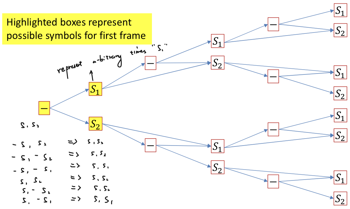
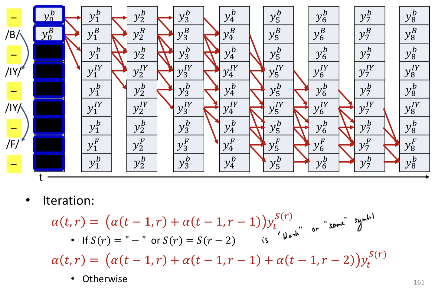
• Solution: Introduce an explicit extra symbol which serves to separate discrete versions of a symbol
  • A “blank” (represented by “-”)
  • RRR---OO---DDD = ROD
  • RR-R---OO---D-DD = RRODD

Modified forward algorithm

• A blank is mandatory between repetitions of a symbol but not required between distinct symbols
• Skips are permitted across a blank, but only if the symbols on either side are different

Modified backward algorithm

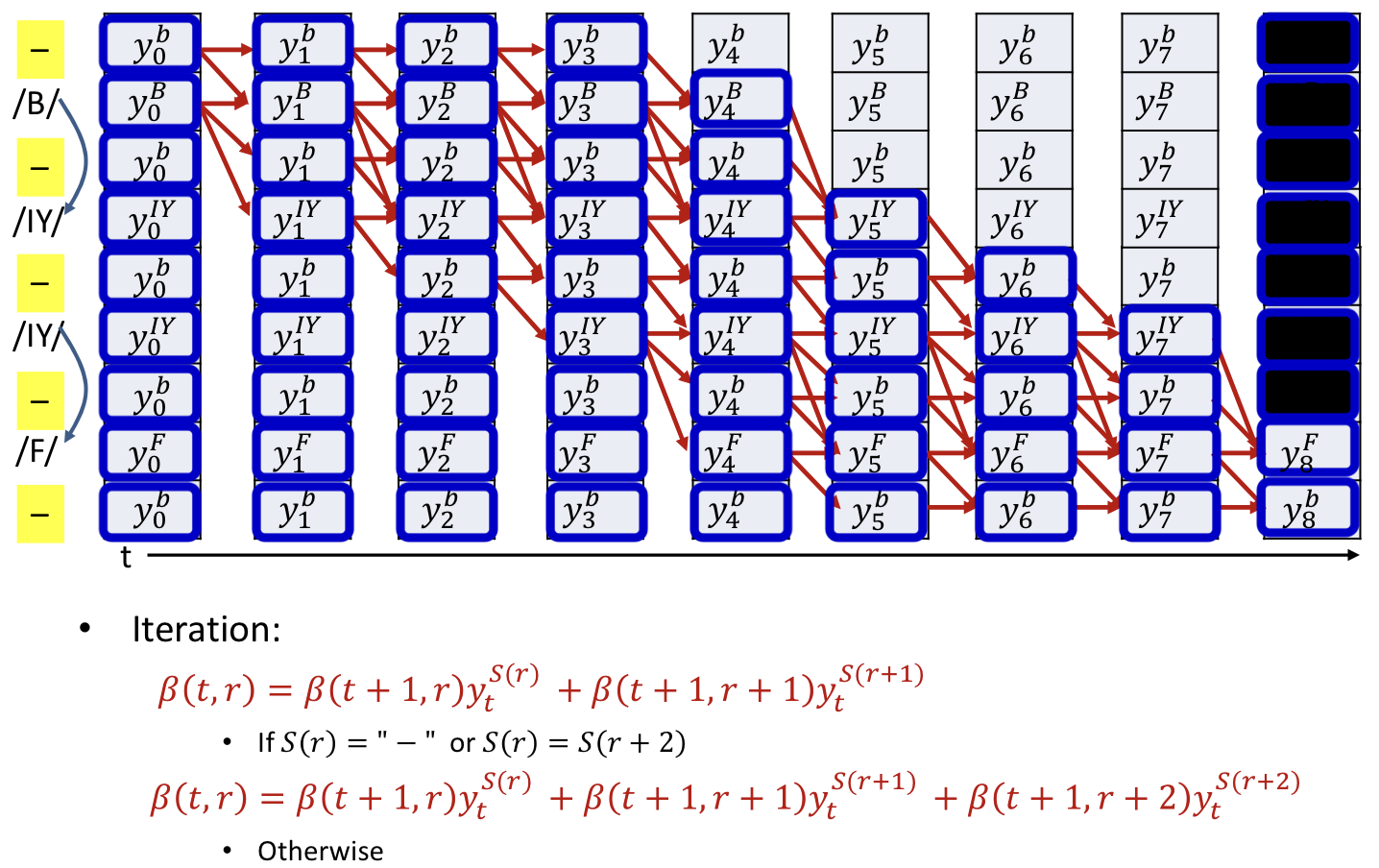
Overall training procedure

1. Setup the network

   • Typically many-layered LSTM

2. Initialize all parameters of the network

   • Include a 「blank」 symbol in vocabulary

3. Foreach training instance

   • Pass the training instance through the network and obtain all symbol probabilities at each time
   • Construct the graph representing the specific symbol sequence in the instance

4. Backword pass

   • Perform the forward backward algorithm to compute $\alpha(t,r)$ and $\beta(t,r)$

   • Compute derivative of divergence $\nabla_{Y_{t}} D I V$ for each $Y_t$

   • $\nabla_{Y_{t}} D I V=\left[\begin{array}{llll}\frac{d D I V}{d y_{t}^{0}} & \frac{d D I V}{d y_{t}^{1}} & \cdots & \frac{d D I V}{d y_{t}^{L-1}}\end{array}\right]$
   • $\frac{d D I V}{d y_{t}^{l}}=-\sum_{r: S(r)=l} \frac{\gamma(t, r)}{y_{t}^{S(r)}}$
   • Aggregate derivatives over minibatch and update parameters

5. CTC: Connectionist Temporal Classification

   • The overall framework is referred to as CTC
   • This is in fact a suboptimal decode that actually finds the most likely time-synchronous output sequence
6. Actual decoding objective
   • $\hat{\mathbf{S}}=\underset{\mathbf{s}}{\operatorname{argmax}} \alpha_{\mathbf{S}}\left(S_{K-1}, T-1\right)$
   • Explicit computation of this will require evaluate of an exponential number of symbol sequences

Beam search

• Only used in test
• Uses breadth-first search to build its search tree
  • Choose top k words for next prediction (prone)

• Reference