Identical to minimizing the KL divergence between the desired output and actual output 1+e−(w0+wTXi)1
MLP
Separable case
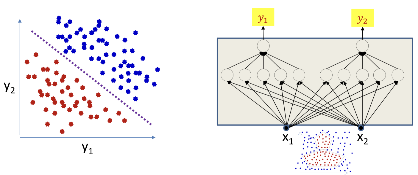
The rest of the network may be viewed as a transformation that transforms data from non-linear classes to linearly separable features
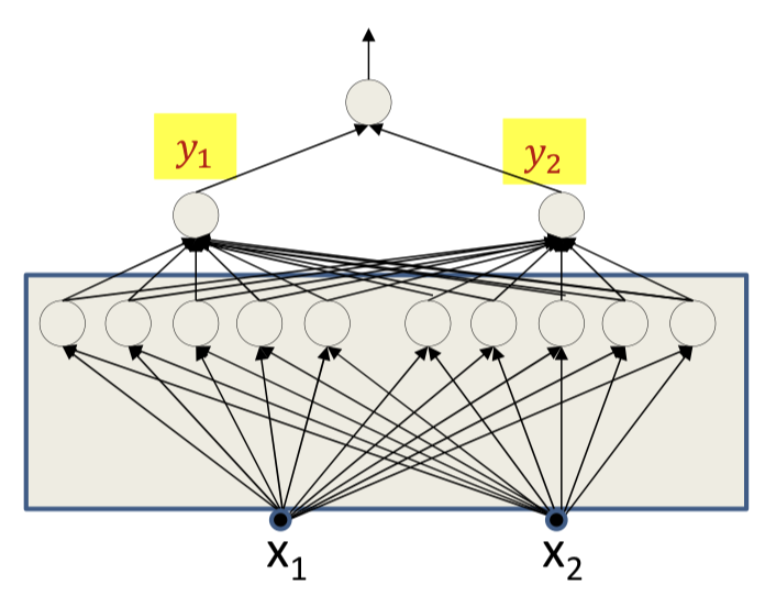
We can now attach any linear classifier above it for perfect classification
Need not be a perceptron
Could even train an SVM on top of the features!
For insufficient structures, the network may attempt to transform the inputs to linearly separable features
Will fail to separate exactly, but will try to minimize error
The network until the second-to-last layer is a non-linear function f(X) that converts the input space X of into the feature space where the classes are maximally linearly separable
Lower layers
Manifold hypothesis: For separable classes, the classes are linearly separable on a non-linear manifold
Layers sequentially “straighten” the data manifold
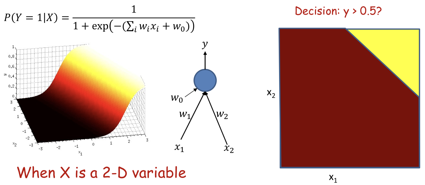
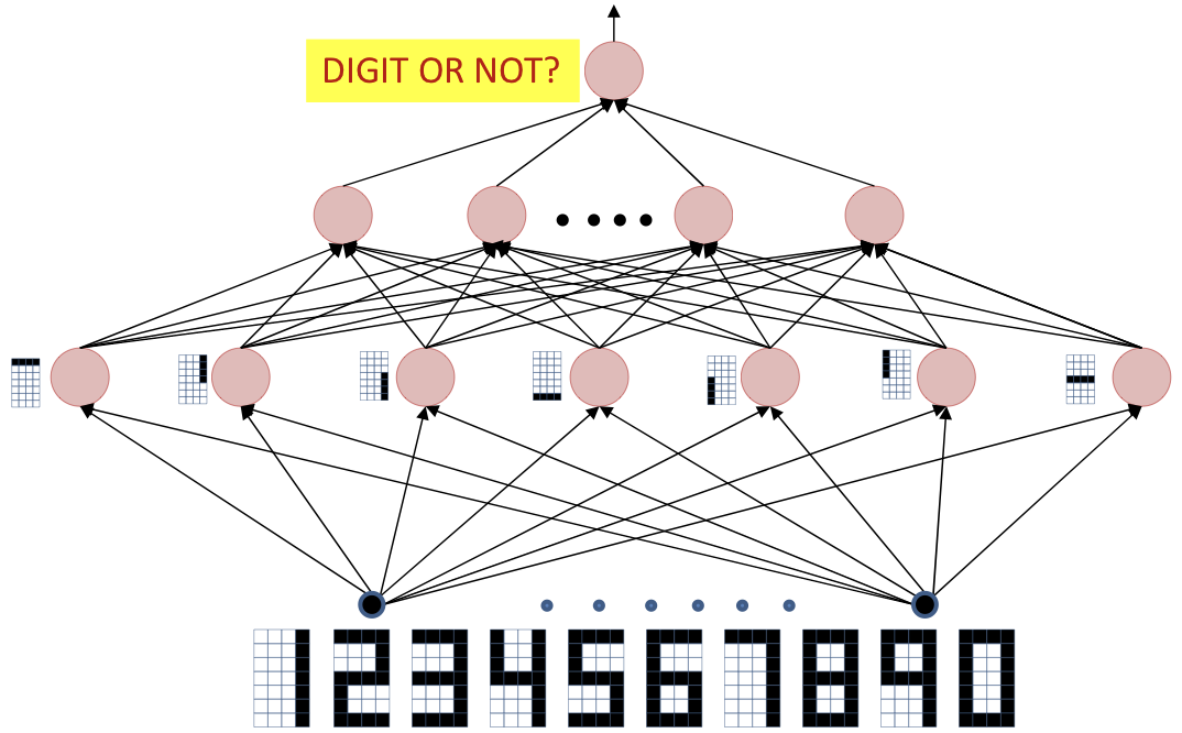
The “feature extraction” layer transforms the data such that the posterior probability may now be modelled by a logistic
Weight as a template
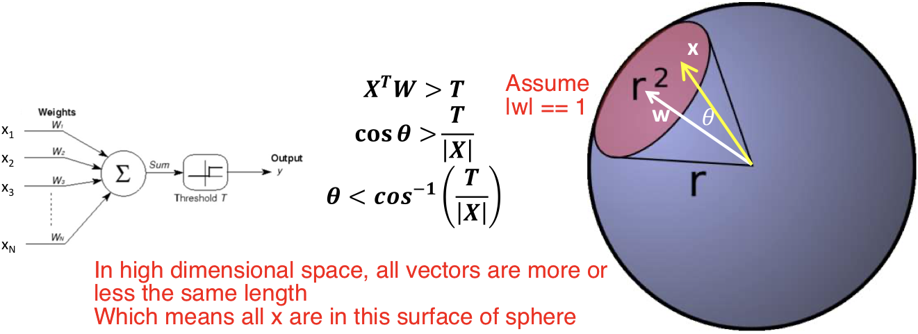
In high dimensional space, all vectors are more or less the same length
Which means all x are in this surface of sphere
The perceptron fires if the input is within a specified angle of the weight
Represents a convex region on the surface of the sphere!
The network is a Boolean function over these regions
Neuron fires if the input vector is close enough to the weight vector
If the input pattern matches the weight pattern closely enough
The perceptron is a correlation filter!
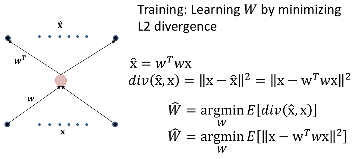
Autoencoder
The lowest layers of a network detect significant features in the signal
The signal could be (partially) reconstructed using these features
Will retain all the significant components of the signal
Simplest autoencoder
This is just PCA!
The autoencoder finds the direction of maximum energy
Simply varying the hidden representation will result in an output that lies along the major axis
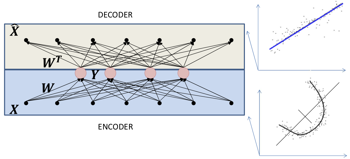
Terminology
Encoder
The “Analysis” net which computes the hidden representation
Decoder
The “Synthesis” which recomposes the data from the hidden representation
Nonlinearity
When the hidden layer has a linear activation the decoder represents the best linear manifold to fit the data
Varying the hidden value will move along this linear manifold
When the hidden layer has non-linear activation, the net performs nonlinear PCA
The decoder represents the best non-linear manifold to fit the data
Varying the hidden value will move along this non-linear manifold
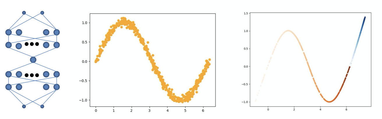
The model is specific to the training data
Varying the hidden layer value only generates data along the learned manifold
Any input will result in an output along the learned manifold
But may not generalize beyond the manifold
Input unseen data may behave beyond intuitive manner, no constrain!
The decoder can only generate data on the manifold that the training data lie on
This also makes it an excellent “generator” of the distribution of the training data
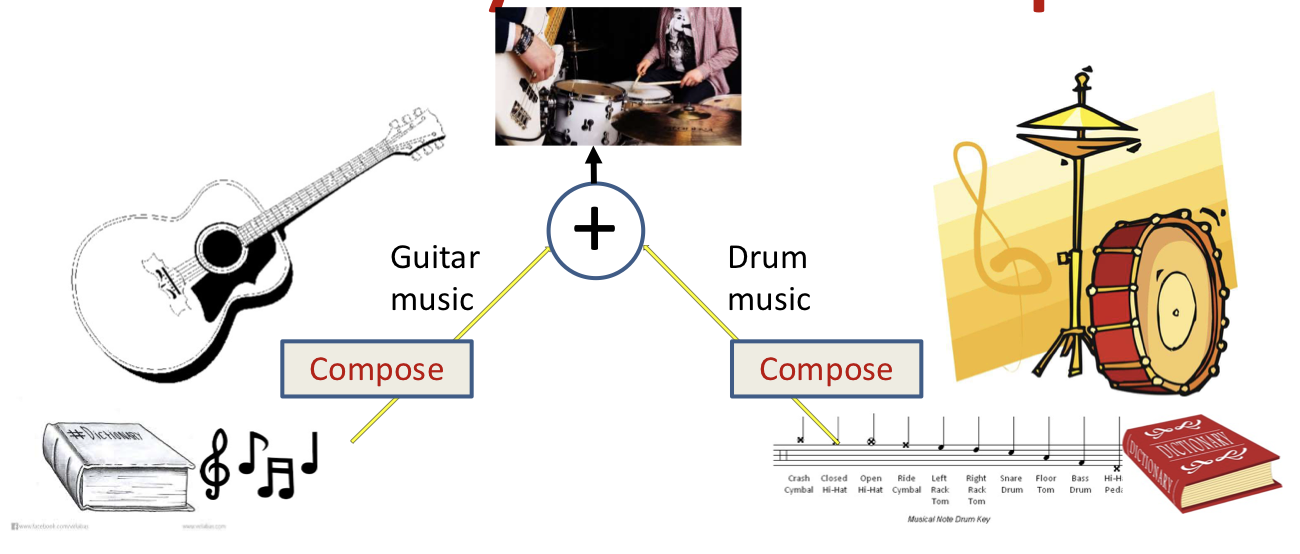
Dictionary-based techniques
The decoder represents a source-specific generative dictionary
Exciting it will produce typical data from the source!
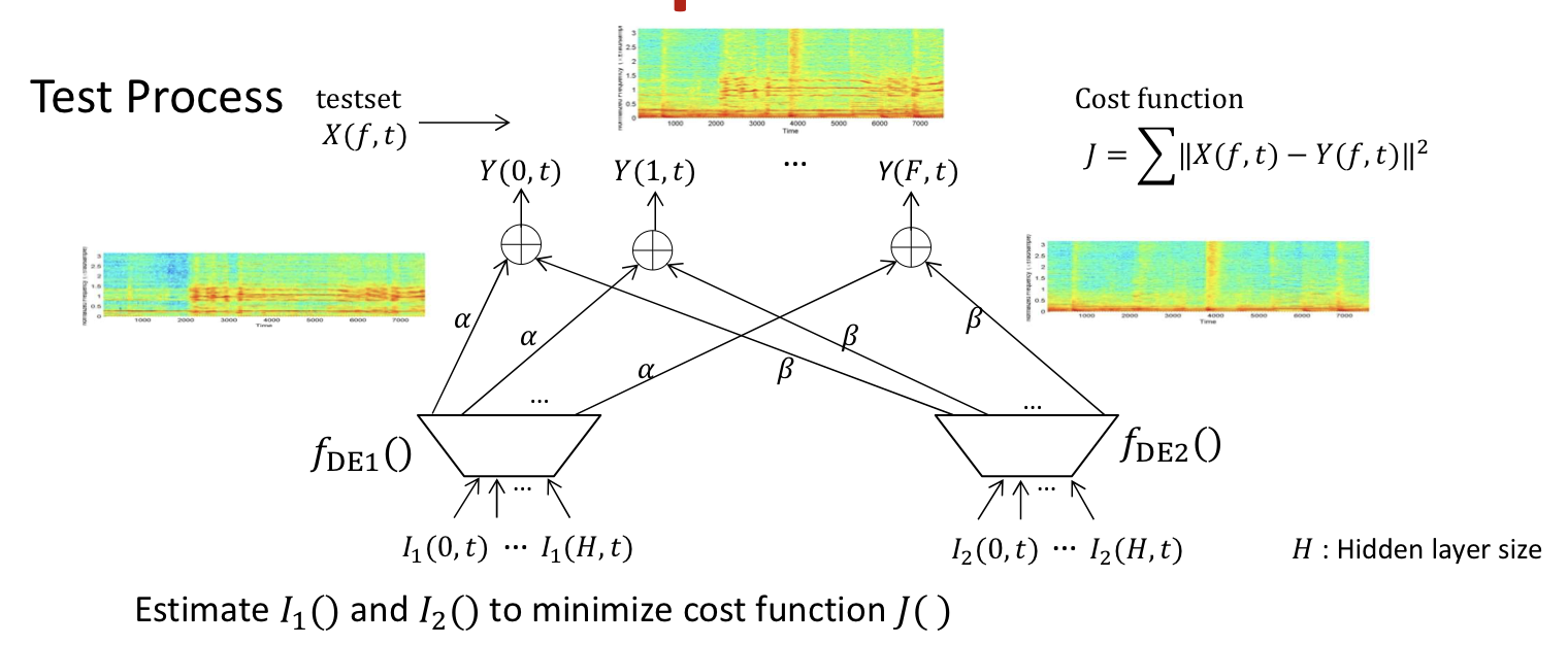
Signal separation
Separation: Identify the combination of entries from both dictionaries that compose the mixed signal
Given mixed signal and source dictionaries, find excitation that best recreates mixed signal