Training hopfield nets

Geometric approach

• Behavior of $\mathbf{E}(\mathbf{y})=\mathbf{y}^{T} \mathbf{W y}$ with $\mathbf{W}=\mathbf{Y} \mathbf{Y}^{T}-N_{p} \mathbf{I}$ is identical to behavior with $W=YY^T$

  • Energy landscape only differs by an additive constant
  • Gradients and location of minima remain same (Have the same eigen vectors)

• Sine : $\mathbf{y}^{T}\left(\mathbf{Y} \mathbf{Y}^{T}-N_{p} \mathbf{I}\right) \mathbf{y}=\mathbf{y}^{T} \mathbf{Y} \mathbf{Y}^{T} \mathbf{y}-N N_{p}$

• We use $\mathbf{y}^{T} \mathbf{Y} \mathbf{Y}^{T} \mathbf{y}$ for analyze

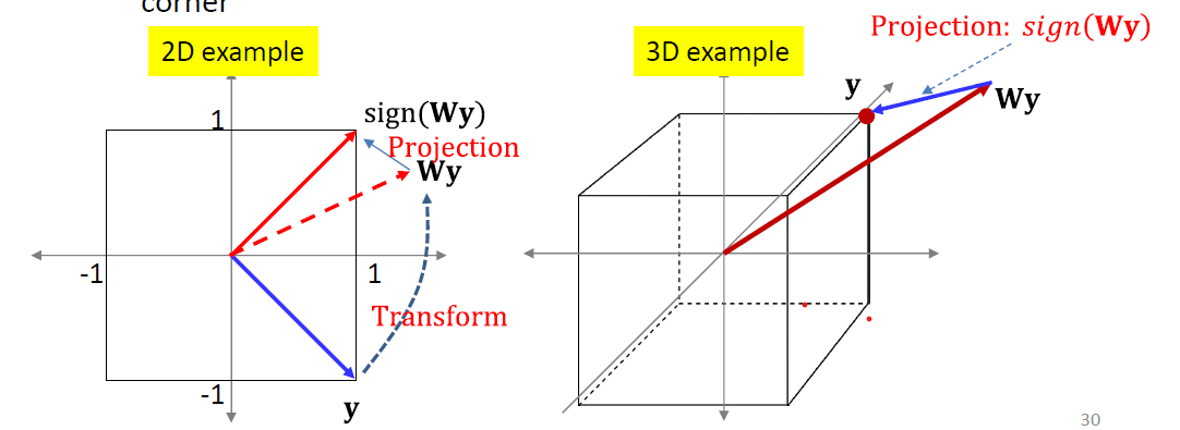
• A pattern $y_p$ is stored if:

  • $\operatorname{sign}\left(\mathbf{W} \mathbf{y}_{p}\right)=\mathbf{y}\_{p}$ for all target patterns

• Training: Design $W$ such that this holds

• Simple solution: $y_p$ is an Eigenvector of $W$

Storing k orthogonal patterns

• Let $\mathbf{Y}=\left[\mathbf{y}\_{1} \mathbf{y}\_{2} \ldots \mathbf{y}\_{K}\right]$
  • $\mathbf{W}=\mathbf{Y} \Lambda \mathbf{Y}^{T}$
  • $\lambda_1,...,\lambda_k$ are positive
  • for $\lambda_1= \lambda_2=\lambda_k= 1$ this is exactly the Hebbian rule
• Any pattern $y$ can be written as
  • $\mathbf{y}=a_{1} \mathbf{y}_{1}+a_{2} \mathbf{y}_{2}+\cdots+a_{N} \mathbf{y}_{N}$
  • $\mathbf{W y}=a_{1} \mathbf{W y}_{1}+a_{2} \mathbf{W y}_{2}+\cdots+a_{N} \mathbf{W y}_{N} = y$
• All patterns are stable
  • Remembers everything
  • Completely useless network
• Even if we store fewer than $N$ patterns
  • Let $Y=\left[\mathbf{y}\_{1} \mathbf{y}\_{2} \ldots \mathbf{y}\_{K} \mathbf{r}\_{K+1} \mathbf{r}\_{K+2} \ldots \mathbf{r}\_{N}\right]$
  • $W=Y \Lambda Y^{T}$
  • $\mathbf{r}\_{K+1} \mathbf{r}\_{K+2} \ldots \mathbf{r}\_{N}$ are orthogonal to $\mathbf{y}_1 \mathbf{y}_2 \ldots \mathbf{y}_K$
  • $\lambda_1= \lambda_2=\lambda_k= 1$
  • Problem arise because eigen values are all 1.0
    • Ensures stationarity of vectors in the subspace
    • All stored patterns are equally important

General (nonorthogonal) vectors

• $w_{j i}=\sum_{p \in\{p\}} y_{i}^{p} y_{j}^{p}$
• The maximum number of stationary patterns is actually exponential in $N$ (McElice and Posner, 84’)
• For a specific set of $K$ patterns, we can always build a network for which all $K$ patterns are stable provided $k \le N$
  • But this may come with many “parasitic” memories

Optimization

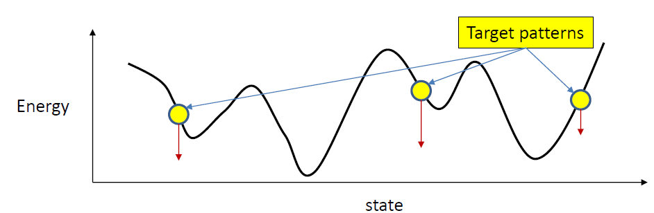
• Energy function
  • $E=-\frac{1}{2} \mathbf{y}^{T} \mathbf{W} \mathbf{y}-\mathbf{b}^{T} \mathbf{y}$
  • This must be maximally low for target patterns
  • Must be maximally high for all other patterns
    • So that they are unstable and evolve into one of the target patterns
• Estimate $W$ such that
  • $E$ is minimized for $y_1,...,y_P$
  • $E$ is maximized for all other $y$
• Minimize total energy of target patterns
  • $E(\mathbf{y})=-\frac{1}{2} \mathbf{y}^{T} \mathbf{W y} \quad \widehat{\mathbf{W}}=\underset{\mathbf{W}}{\operatorname{argmin}} \sum_{\mathbf{y} \in \mathbf{Y}_{P}} E(\mathbf{y})$
  • However, might also pull all the neighborhood states down
• Maximize the total energy of all non-target patterns
  • $E(\mathbf{y})=-\frac{1}{2} \mathbf{y}^{T} \mathbf{W} \mathbf{y}$
  • $\widehat{\mathbf{W}}=\underset{\mathbf{W}}{\operatorname{argmin}} \sum_{\mathbf{y} \in \mathbf{Y}_{P}} E(\mathbf{y})-\sum_{\mathbf{y} \notin \mathbf{Y}_{P}} E(\mathbf{y})$
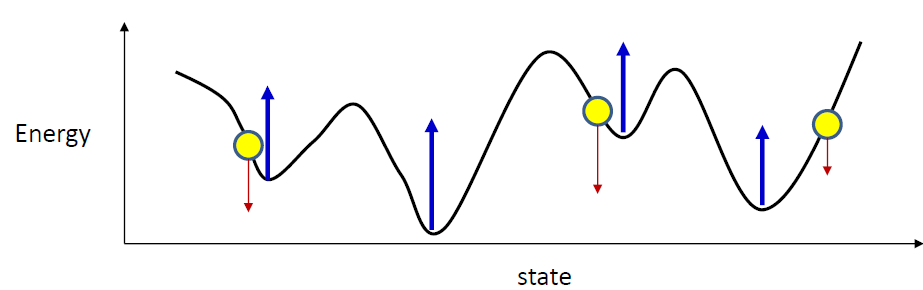
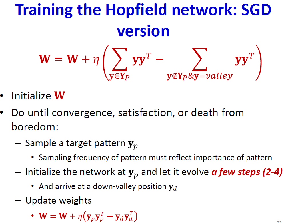
• Simple gradient descent
  • $\mathbf{W}=\mathbf{w}+\eta\left(\sum_{\mathbf{y} \in \mathbf{Y}_{P}} \mathbf{y} \mathbf{y}^{T}-\sum_{\mathbf{y} \notin \mathbf{Y}_{P}} \mathbf{y} \mathbf{y}^{T}\right)$
  • minimize the energy at target patterns
    • 
  • raise all non-target patterns
    • Do we need to raise everything?

Raise negative class

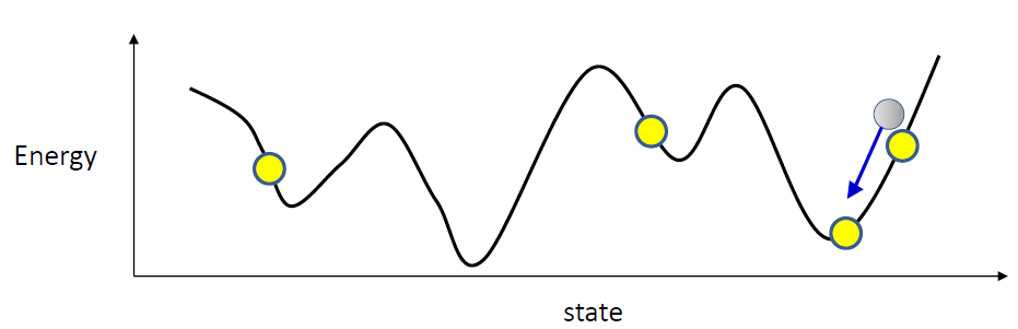
• Focus on raising the valleys
  • If you raise every valley, eventually they’ll all move up above the target patterns, and many will even vanish
  • 
• How do you identify the valleys for the current $W$?
  • 
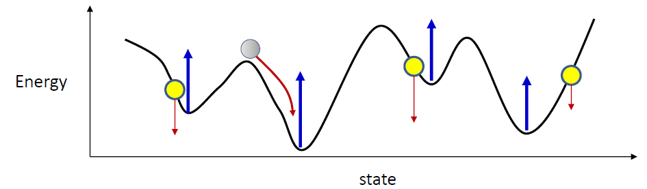
  • Initialize the network randomly and let it evolve
  • It will settle in a valley

• Should we randomly sample valleys?
  • Are all valleys equally important?
  • Major requirement: memories must be stable
    • They must be broad valleys
  • 
• Solution: initialize the network at valid memories and let it evolve
  • It will settle in a valley
  • If this is not the target pattern, raise it
• What if there’s another target pattern downvalley
  • 
  • no need to raise the entire surface, or even every valley
    • Raise the neighborhood of each target memory
• 

Storing more than N patterns

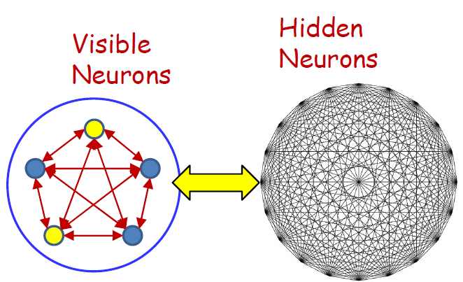
• Visible neurons
  • The neurons that store the actual patterns of interest
• Hidden neurons
  • The neurons that only serve to increase the capacity but whose actual values are not important

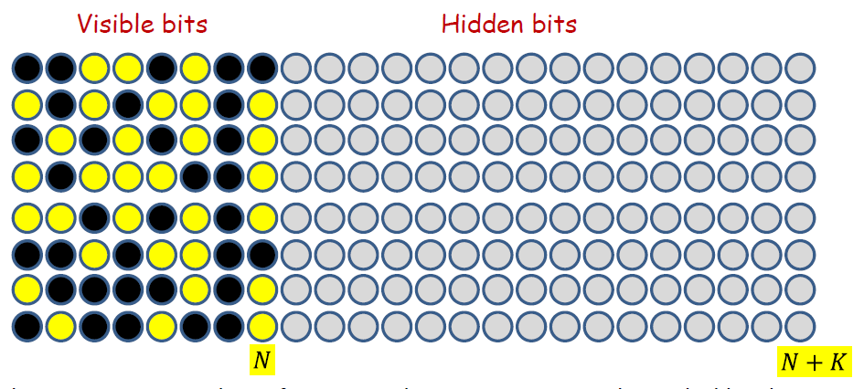
• The maximum number of patterns the net can store is bounded by the width $N$ of the patterns..
• So lets pad the patterns with $K$ “don’t care” bits
  • The new width of the patterns is $N+K$
  • Now we can store $N+K$ patterns!
• Taking advantage of don’t care bits
  • Simple random setting of don’t care bits, and using the usual training and recall strategies for Hopfield nets should work
  • However, to exploit it properly, it helps to view the Hopfield net differently: as a probabilistic machine

A probabilistic interpretation

• For binary y the energy of a pattern is the analog of the negative log likelihood of a Boltzmann distribution
  • Minimizing energy maximizes log likelihood
  • $E(\mathbf{y})=-\frac{1}{2} \mathbf{y}^{T} \mathbf{W y} \quad P(\mathbf{y})=\operatorname{Cexp}(-E(\mathbf{y}))$

Boltzmann Distribution

• $E(\mathbf{y})=-\frac{1}{2} \mathbf{y}^{T} \mathbf{W} \mathbf{y}-\mathbf{b}^{T} \mathbf{y}$
• $P(\mathbf{y})=\operatorname{Cexp}\left(\frac{-E(\mathbf{y})}{k T}\right)$
• $C=\frac{1}{\sum_{\mathrm{y}} \exp \left(\frac{-E(\mathbf{y})}{k T}\right)}$
• $k$ is the Boltzmann constant, $T$ is the temperature of the system
• Optimizing $W$
  • $E(\mathbf{y})=-\frac{1}{2} \mathbf{y}^{T} \mathbf{W} \mathbf{y} \quad \widehat{\mathbf{W}}=\underset{\mathbf{W}}{\operatorname{argmin}} \sum_{\mathbf{y} \in \mathbf{Y}_{P}} E(\mathbf{y})-\sum_{\mathbf{y} \notin \mathbf{Y}_{P}} E(\mathbf{y})$
  • Simple gradient descent
  • $\mathbf{W}=\mathbf{W}+\eta\left(\sum_{\mathbf{y} \in \mathbf{Y}_{P}} \alpha_{\mathbf{y}} \mathbf{y} \mathbf{y}^{T}-\sum_{\mathbf{y} \notin \mathbf{Y}_{P}} \beta(E(\mathbf{y})) \mathbf{y} \mathbf{y}^{T}\right)$
  • $\alpha_y$ more importance to more frequently presented memories
  • $\beta (E(y))$ more importance to more attractive spurious memories
  • Looks like an expectation
  • $\mathbf{W}=\mathbf{W}+\eta\left(E_{\mathbf{y} \sim \mathbf{Y}_{P}} \mathbf{y} \mathbf{y}^{T}-E_{\mathbf{y} \sim Y} \mathbf{y} \mathbf{y}^{T}\right)$
• The behavior of the Hopfield net is analogous to annealed dynamics of a spin glass characterized by a Boltzmann distribution