This lecture redefined a regular Hopfield net as a **stochastic** system: Boltzmann machines. And talked about the training, sampling issues of Boltzmann machines model, introduced *Restricted* Boltzmann Machines, which is a common used model in practice.
The Hopfield net as a distribution
The Helmholtz Free Energy of a System
At any time, the probability of finding the system in state s s s T T T P T ( s ) P_T(s) P T ( s )
At each state it has a potential energy E s E_s E s
The internal energy of the system, representing its capacity to do work, is the average
U T = ∑ S P T ( s ) E S
U_{T}=\sum_{S} P_{T}(s) E_{S}
U T = S ∑ P T ( s ) E S
The capacity to do work is counteracted by the internal disorder of the system, i.e. its entropy
H T = − ∑ S P T ( s ) log P T ( s )
H_{T}=-\sum_{S} P_{T}(s) \log P_{T}(s)
H T = − S ∑ P T ( s ) log P T ( s )
The Helmholtz free energy of the system measures the useful work derivable from it and combines the two terms
F T = U T + k T H T
F_{T}=U_{T}+k T H_{T}
F T = U T + k T H T = ∑ S P T ( s ) E S − k T ∑ S P T ( s ) log P T ( s )
=\sum_{S} P_{T}(s) E_{S}-k T \sum_{S} P_{T}(s) \log P_{T}(s)
= S ∑ P T ( s ) E S − k T S ∑ P T ( s ) log P T ( s )
The probability distribution of the states at steady state is known as the Boltzmann distribution
Minimizing this w.r.t P T ( s ) P_T(s) P T ( s )
P T ( s ) = 1 Z exp ( − E S k T )
P_{T}(s)=\frac{1}{Z} \exp \left(\frac{-E_{S}}{k T}\right)
P T ( s ) = Z 1 exp ( k T − E S )
Z Z Z
Hopfield net as a distribution
E ( S ) = − ∑ i < j w i j s i s j − b i s i E(S)=-\sum_{i<j} w_{i j} s_{i} s_{j}-b_{i} s_{i} E ( S ) = − ∑ i < j w i j s i s j − b i s i P ( S ) = exp ( − E ( S ) ) ∑ S ′ exp ( − E ( S ′ ) ) P(S)=\frac{\exp (-E(S))}{\sum_{S^{\prime}} \exp \left(-E\left(S^{\prime}\right)\right)} P ( S ) = ∑ S ′ exp ( − E ( S ′ ) ) exp ( − E ( S ) ) The stochastic Hopfield network models a probability distribution over states
It is a generative model: generates states according to P ( S ) P(S) P ( S )
The field at a single node
Let's take one node as example
Let S S S S ′ S^\prime S ′
P ( S ) = P ( s i = 1 ∣ s j ≠ i ) P ( s j ≠ i ) P(S)=P\left(s_{i}=1 \mid s_{j \neq i}\right) P\left(s_{j \neq i}\right) P ( S ) = P ( s i = 1 ∣ s j ≠ i ) P ( s j ≠ i ) P ( S ′ ) = P ( s i = − 1 ∣ s j ≠ i ) P ( s j ≠ i ) P\left(S^{\prime}\right)=P\left(s_{i}=-1 \mid s_{j \neq i}\right) P\left(s_{j \neq i}\right) P ( S ′ ) = P ( s i = − 1 ∣ s j ≠ i ) P ( s j ≠ i ) log P ( S ) − log P ( S ′ ) = log P ( s i = 1 ∣ s j ≠ i ) − log P ( s i = − 1 ∣ s j ≠ i ) \log P(S)-\log P\left(S^{\prime}\right)=\log P\left(s_{i}=1 \mid s_{j \neq i}\right)-\log P\left(s_{i}=-1 \mid s_{j \neq i}\right) log P ( S ) − log P ( S ′ ) = log P ( s i = 1 ∣ s j ≠ i ) − log P ( s i = − 1 ∣ s j ≠ i ) log P ( S ) − log P ( S ′ ) = log P ( s i = 1 ∣ s j ≠ i ) 1 − P ( s i = 1 ∣ s j ≠ i ) \log P(S)-\log P\left(S^{\prime}\right)=\log \frac{P\left(s_{i}=1 \mid s_{j \neq i}\right)}{1-P\left(s_{i}=1 \mid s_{j \neq i}\right)} log P ( S ) − log P ( S ′ ) = log 1 − P ( s i = 1 ∣ s j ≠ i ) P ( s i = 1 ∣ s j ≠ i )
log P ( S ) = − E ( S ) + C \log P(S)=-E(S)+C log P ( S ) = − E ( S ) + C
E ( S ) = − 1 2 ( E not i + ∑ j ≠ i w i j s j + b i ) E(S)=-\frac{1}{2}\left(E_{\text {not } i}+\sum_{j \neq i} w_{i j} s_{j}+b_{i}\right) E ( S ) = − 2 1 ( E not i + ∑ j ≠ i w i j s j + b i ) E ( S ′ ) = − 1 2 ( E not i − ∑ j ≠ i w i j s j − b i ) E\left(S^{\prime}\right)=-\frac{1}{2}\left(E_{\text {not } i}-\sum_{j \neq i} w_{i j} s_{j}-b_{i}\right) E ( S ′ ) = − 2 1 ( E not i − ∑ j ≠ i w i j s j − b i )
log P ( S ) − log P ( S ′ ) = E ( S ′ ) − E ( S ) = ∑ j ≠ i w i j S j + b i \log P(S)-\log P\left(S^{\prime}\right)=E\left(S^{\prime}\right)-E(S)=\sum_{j \neq i} w_{i j} S_{j}+b_{i} log P ( S ) − log P ( S ′ ) = E ( S ′ ) − E ( S ) = ∑ j ≠ i w i j S j + b i
log ( P ( s i = 1 ∣ s j ≠ i ) 1 − P ( s i = 1 ∣ s j ≠ i ) ) = ∑ j ≠ i w i j s j + b i \log \left(\frac{P\left(s_{i}=1 \mid s_{j \neq i}\right)}{1-P\left(s_{i}=1 \mid s_{j \neq i}\right)}\right)=\sum_{j \neq i} w_{i j} s_{j}+b_{i} log ( 1 − P ( s i = 1 ∣ s j ≠ i ) P ( s i = 1 ∣ s j ≠ i ) ) = ∑ j ≠ i w i j s j + b i
P ( s i = 1 ∣ s j ≠ i ) = 1 1 + e − ( ∑ j ≠ i w i j s j + b i ) P\left(s_{i}=1 \mid s_{j \neq i}\right)=\frac{1}{1+e^{-\left(\sum_{j \neq i} w_{i j} s_{j}+b_{i}\right)}} P ( s i = 1 ∣ s j ≠ i ) = 1 + e − ( ∑ j ≠ i w i j s j + b i ) 1
The probability of any node taking value 1 given other node values is a logistic
Redefining the network
Redefine a regular Hopfield net as a stochastic system
Each neuron is now a stochastic unit with a binary state s i s_i s i
z i = ∑ j w i j s j + b i z_{i}=\sum_{j} w_{i j} s_{j}+b_{i} z i = ∑ j w i j s j + b i P ( s i = 1 ∣ s j ≠ i ) = 1 1 + e − z i P\left(s_{i}=1 \mid s_{j \neq i}\right)=\frac{1}{1+e^{-z_{i}}} P ( s i = 1 ∣ s j ≠ i ) = 1 + e − z i 1
Note
The Hopfield net is a probability distribution over binary sequences (Boltzmann distribution)
The conditional distribution of individual bits in the sequence is a logistic
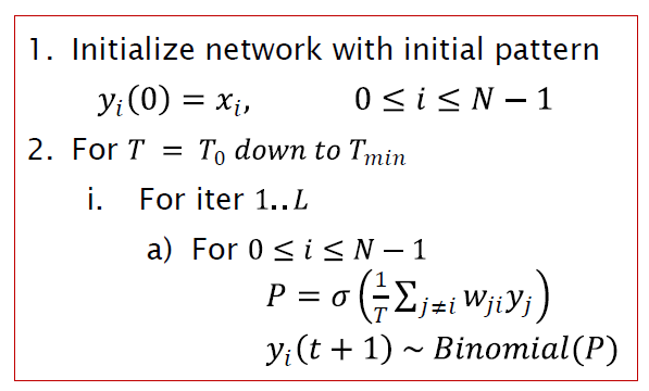
The evolution of the Hopfield net can be made stochastic
Instead of deterministically responding to the sign of the local field, each neuron responds probabilistically
Recall patterns
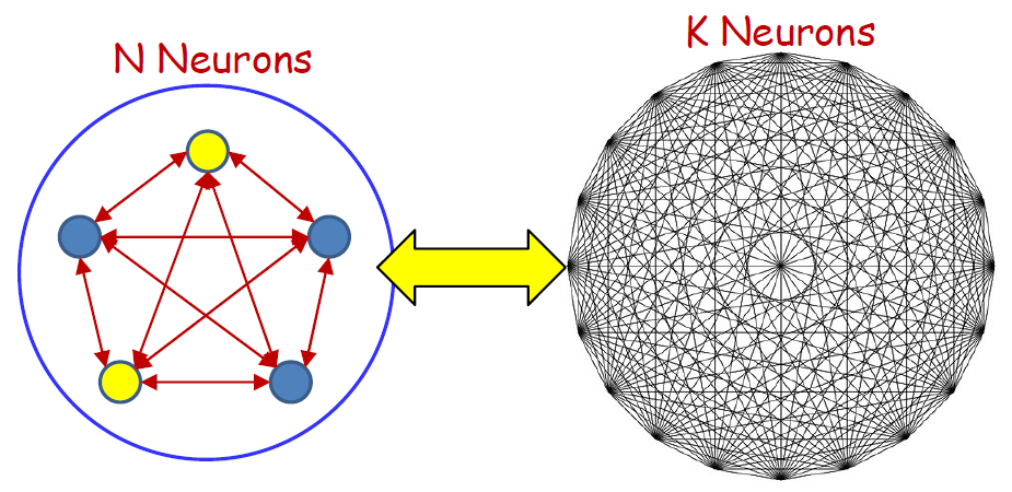
The Boltzmann Machine
The entire model can be viewed as a generative model
Has a probability of producing any binary vector y y y
E ( y ) = − 1 2 y T W y E(\mathbf{y})=-\frac{1}{2} \mathbf{y}^{T} \mathbf{W} \mathbf{y} E ( y ) = − 2 1 y T W y P ( y ) = Cexp ( − E ( y ) T ) P(\mathbf{y})=\operatorname{Cexp}\left(-\frac{E(\mathbf{y})}{T}\right) P ( y ) = Cexp ( − T E ( y ) )
Training a Hopfield net: Must learn weights to “remember ” target states and “dislike ” other states
Must learn weights to assign a desired probability distribution to states
Just maximize likelihood
Maximum Likelihood Training
log ( P ( S ) ) = ( ∑ i < j w i j s i s j ) − log ( ∑ S ′ exp ( ∑ i < j w i j s i ′ s j ′ ) ) \log (P(S))=\left(\sum_{i<j} w_{i j} s_{i} s_{j}\right)-\log \left(\sum_{S^{\prime}} \exp \left(\sum_{i<j} w_{i j} s_{i}^{\prime} s_{j}^{\prime}\right)\right) log ( P ( S ) ) = ( ∑ i < j w i j s i s j ) − log ( ∑ S ′ exp ( ∑ i < j w i j s i ′ s j ′ ) ) L = 1 N ∑ S ∈ S log ( P ( S ) ) = 1 N ∑ S ( ∑ i < j w i j s i s j ) − log ( ∑ S ′ exp ( ∑ i < j w i j s i ′ s j ′ ) ) \mathcal{L}=\frac{1}{N} \sum_{S \in \mathbf{S}} \log (P(S)) =\frac{1}{N} \sum_{S}\left(\sum_{i<j} w_{i j} s_{i} s_{j}\right)-\log \left(\sum_{S^{\prime}} \exp \left(\sum_{i<j} w_{i j} s_{i}^{\prime} s_{j}^{\prime}\right)\right) L = N 1 ∑ S ∈ S log ( P ( S ) ) = N 1 ∑ S ( ∑ i < j w i j s i s j ) − log ( ∑ S ′ exp ( ∑ i < j w i j s i ′ s j ′ ) ) Second term derivation
d log ( ∑ S ′ exp ( ∑ i < j w i j s i ′ s j ′ ) ) d w i j = ∑ S ′ exp ( ∑ i < j w i j s i ′ s j ′ ) ∑ S ′ exp ( ∑ i < j w i j s i ′ ′ s j ′ ) s i ′ s j ′ \frac{d \log \left(\sum_{S^{\prime}} \exp \left(\sum_{i<j} w_{i j} s_{i}^{\prime} s_{j}^{\prime}\right)\right)}{d w_{i j}}=\sum_{S^{\prime}} \frac{\exp \left(\sum_{i<j} w_{i j} s_{i}^{\prime} s_{j}^{\prime}\right)}{\sum_{S^{\prime}} \exp \left(\sum_{i<j} w_{i j} s_{i}^{\prime \prime} s_{j}^{\prime}\right)} s_{i}^{\prime} s_{j}^{\prime} d w i j d log ( ∑ S ′ exp ( ∑ i < j w i j s i ′ s j ′ ) ) = ∑ S ′ ∑ S ′ exp ( ∑ i < j w i j s i ′ ′ s j ′ ) exp ( ∑ i < j w i j s i ′ s j ′ ) s i ′ s j ′ d log ( ∑ S ′ exp ( ∑ i < j w i j s i ′ s j ′ ) ) d w i j = ∑ S ′ P ( S ′ ) s i ′ s j ′ \frac{d \log \left(\sum_{S^{\prime}} \exp \left(\sum_{i<j} w_{i j} s_{i}^{\prime} s_{j}^{\prime}\right)\right)}{d w_{i j}}=\sum_{S_{\prime}} P\left(S^{\prime}\right) s_{i}^{\prime} s_{j}^{\prime} d w i j d log ( ∑ S ′ exp ( ∑ i < j w i j s i ′ s j ′ ) ) = ∑ S ′ P ( S ′ ) s i ′ s j ′ The second term is simply the expected value of s i S j s_iS_j s i S j
We cannot compute it exhaustively, but we can compute it by sampling!
Overall gradient ascent rule
w i j = w i j + η d ⟨ log ( P ( S ) ) ⟩ d w i j w_{i j}=w_{i j}+\eta \frac{d\langle\log (P(\mathbf{S}))\rangle}{d w_{i j}} w i j = w i j + η d w i j d ⟨ log ( P ( S ) ) ⟩
Overall Training
Initialize weights
Let the network run to obtain simulated state samples Compute gradient and update weights
Iterate
Note the similarity to the update rule for the Hopfield network
The only difference is how we got the samples
Adding Capacity
Visible neurons
The neurons that store the actual patterns of interest
Hidden neurons
The neurons that only serve to increase the capacity but whose actual values are not important
We could have multiple hidden patterns coupled with any visible pattern
These would be multiple stored patterns that all give the same visible output
We are interested in the marginal probabilities
S = ( V , H ) S=(V,H) S = ( V , H ) P ( S ) = exp ( − E ( S ) ) ∑ S ′ exp ( − E ( S ′ ) ) P(S)=\frac{\exp (-E(S))}{\sum_{S^{\prime}} \exp \left(-E\left(S^{\prime}\right)\right)} P ( S ) = ∑ S ′ exp ( − E ( S ′ ) ) exp ( − E ( S ) ) P ( S ) = P ( V , H ) P(S) = P(V,H) P ( S ) = P ( V , H ) P ( V ) = ∑ H P ( S ) P(V)=\sum_{H} P(S) P ( V ) = ∑ H P ( S )
Train to maximize probability of desired patterns of visible bits
E ( S ) = − ∑ i < j w i j s i s j E(S)=-\sum_{i<j} w_{i j} s_{i} s_{j} E ( S ) = − ∑ i < j w i j s i s j P ( S ) = exp ( ∑ i < j w i j s i s j ) ∑ S ′ exp ( ∑ i < j w i j s i ′ s j ′ ) P(S)=\frac{\exp \left(\sum_{i<j} w_{i j} s_{i} s_{j}\right)}{\sum_{S^{\prime}} \exp \left(\sum_{i<j} w_{i j} s_{i}^{\prime} s_{j}^{\prime}\right)} P ( S ) = ∑ S ′ exp ( ∑ i < j w i j s i ′ s j ′ ) exp ( ∑ i < j w i j s i s j ) P ( V ) = ∑ H exp ( ∑ i < j w i j s i s j ) ∑ S ′ exp ( ∑ i < j w i j s i ′ s j ′ ) P(V)=\sum_{H} \frac{\exp \left(\sum_{i<j} w_{i j} s_{i} s_{j}\right)}{\sum_{S^{\prime}} \exp \left(\sum_{i<j} w_{i j} s_{i}^{\prime} s_{j}^{\prime}\right)} P ( V ) = ∑ H ∑ S ′ exp ( ∑ i < j w i j s i ′ s j ′ ) exp ( ∑ i < j w i j s i s j )
Maximum Likelihood Training
log ( P ( V ) ) = log ( ∑ H exp ( ∑ i < j w i j s i s j ) ) − log ( ∑ S ′ exp ( ∑ i < j w i j s i ′ s j ′ ) ) \log (P(V))=\log \left(\sum_{H} \exp \left(\sum_{i<j} w_{i j} s_{i} s_{j}\right)\right)-\log \left(\sum_{S_{\prime}} \exp \left(\sum_{i<j} w_{i j} s_{i}^{\prime} s_{j}^{\prime}\right)\right) log ( P ( V ) ) = log ( H ∑ exp ( i < j ∑ w i j s i s j ) ) − log ( S ′ ∑ exp ( i < j ∑ w i j s i ′ s j ′ ) )
L = 1 N ∑ V ∈ V log ( P ( V ) ) \mathcal{L}=\frac{1}{N} \sum_{V \in \mathbf{V}} \log (P(V)) L = N 1 V ∈ V ∑ log ( P ( V ) ) d L d w i j = 1 N ∑ V ∈ V ∑ H P ( S ∣ V ) s i s j − ∑ S ! P ( S ′ ) s i ′ s j ′
\frac{d \mathcal{L}}{d w_{i j}}=\frac{1}{N} \sum_{V \in \mathbf{V}} \sum_{H} P(S \mid V) s_{i} s_{j}-\sum_{S !} P\left(S^{\prime}\right) s_{i}^{\prime} s_{j}^{\prime}
d w i j d L = N 1 V ∈ V ∑ H ∑ P ( S ∣ V ) s i s j − S ! ∑ P ( S ′ ) s i ′ s j ′
∑ H P ( S ∣ V ) s i s j ≈ 1 K ∑ H ∈ H s i m u l s i S j \sum_{H} P(S \mid V) s_{i} s_{j} \approx \frac{1}{K} \sum_{H \in \mathbf{H}_{s i m u l}} s_{i} S_{j} ∑ H P ( S ∣ V ) s i s j ≈ K 1 ∑ H ∈ H s i m u l s i S j
Computed as the average sampled hidden state with the visible bits fixed
∑ S ′ P ( S ′ ) s i ′ s j ′ ≈ 1 M ∑ S i ∈ S s i m u l s i ′ S j ′ \sum_{S^{\prime}} P\left(S^{\prime}\right) s_{i}^{\prime} s_{j}^{\prime} \approx \frac{1}{M} \sum_{S_{i} \in \mathbf{S}_{s i m u l}} s_{i}^{\prime} S_{j}^{\prime} ∑ S ′ P ( S ′ ) s i ′ s j ′ ≈ M 1 ∑ S i ∈ S s i m u l s i ′ S j ′
Computed as the average of sampled states when the network is running “freely ”
Training
Step1
For each training pattern V i V_i V i
Fix the visible units to V i V_i V i
Let the hidden neurons evolve from a random initial point to generate H i H_i H i
Generate S i = [ V i , H i ] S_i = [V_i,H_i] S i = [ V i , H i ]
Repeat K times to generate synthetic training
S = { S 1 , 1 , S 1 , 2 , … , S 1 K , S 2 , 1 , … , S N , K }
\mathbf{S}=\{S_{1,1}, S_{1,2}, \ldots, S_{1 K}, S_{2,1}, \ldots, S_{N, K}\}
S = { S 1 , 1 , S 1 , 2 , … , S 1 K , S 2 , 1 , … , S N , K }
Step2
Now unclamp the visible units and let the entire network evolve several times to generate
S s i m u l = S _ s i m u l , 1 , S _ s i m u l , 2 , … , S _ s i m u l , M
\mathbf{S}_{simul}=S\_{simul, 1}, S\_{simul, 2}, \ldots, S\_{simul, M}
S s i m u l = S _ s i m u l , 1 , S _ s i m u l , 2 , … , S _ s i m u l , M
Gradients
d ⟨ log ( P ( S ) ) ⟩ d w i j = 1 N K ∑ S s i s j − 1 M ∑ S i ∈ S simul s i ′ s j ′
\frac{d\langle\log (P(\mathbf{S}))\rangle}{d w_{i j}}=\frac{1}{N K} \sum_{\boldsymbol{S}} s_{i} s_{j}-\frac{1}{M} \sum_{S_{i} \in \mathbf{S}_{\text {simul }}} s_{i}^{\prime} s_{j}^{\prime}
d w i j d ⟨ log ( P ( S ) ) ⟩ = N K 1 S ∑ s i s j − M 1 S i ∈ S simul ∑ s i ′ s j ′
w i j = w i j − η d ⟨ log ( P ( S ) ) ⟩ d w i j
w_{i j}=w_{i j}-\eta \frac{d\langle\log (P(\mathbf{S}))\rangle}{d w_{i j}}
w i j = w i j − η d w i j d ⟨ log ( P ( S ) ) ⟩
Gradients are computed as before, except that the first term is now computed over the expanded training data
Issues
Training takes for ever
Doesn’t really work for large problems
A small number of training instances over a small number of bits
Restricted Boltzmann Machines
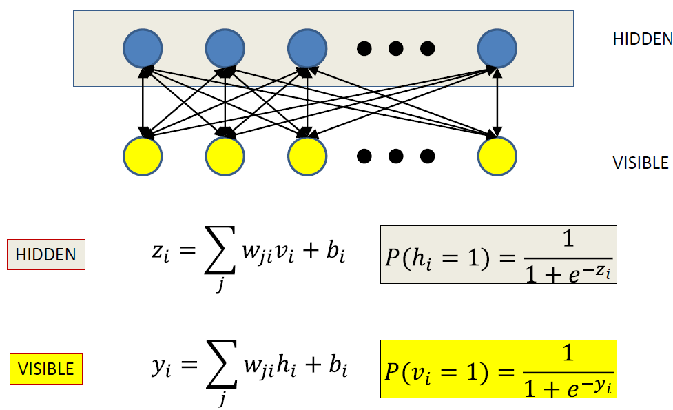
Partition visible and hidden units
Visible units ONLY talk to hidden units
Hidden units ONLY talk to visible units
Training
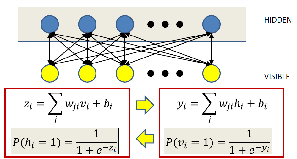
Step1
For each sample
Anchor visible units
Sample from hidden units
No looping!!
Step2
Now unclamp the visible units and let the entire network evolve several times to generate
S s i m u l = S _ s i m u l , 1 , S _ s i m u l , 2 , … , S _ s i m u l , M
\mathbf{S}_{simul}=S\_{simul, 1}, S\_{simul, 2}, \ldots, S\_{simul, M}
S s i m u l = S _ s i m u l , 1 , S _ s i m u l , 2 , … , S _ s i m u l , M
For each sample
Initialize V 0 V_0 V 0
Iteratively generate hidden and visible units
Gradient
∂ log p ( v ) ∂ w i j = < v i h j > 0 − < v i h j > ∞
\frac{\partial \log p(v)}{\partial w_{i j}}=<v_{i} h_{j}>^{0}-<v_{i} h_{j}>^{\infty}
∂ w i j ∂ log p ( v ) = < v i h j > 0 − < v i h j > ∞
A Shortcut: Contrastive Divergence
Recall: Raise the neighborhood of each target memorySufficient to run one iteration to give a good estimate of the gradient
∂ log p ( v ) ∂ w i j = < v i h j > 0 − < v i h j > 1
\frac{\partial \log p(v)}{\partial w_{i j}}=< v_{i} h_{j}>^{0}-<v_{i} h_{j}>^{1}
∂ w i j ∂ log p ( v ) = < v i h j > 0 − < v i h j > 1


