This lecture introduced EM algorithm: an iterative technique to estimate probaility models for missing data. Meanwhile, mixture Gaussian, PCA and factor analysis are actually *generative* models in a way of EM.
Key points
- EM: An iterative technique to estimate probability models for data with missing components or information
- By iteratively “completing” the data and reestimating parameters
- PCA: Is actually a generative model for Gaussian data
- Data lie close to a linear manifold, with orthogonal noise
- A lienar autoencoder!
- Factor Analysis: Also a generative model for Gaussian data
- Data lie close to a linear manifold
- Like PCA, but without directional constraints on the noise (not necessarily orthogonal)
Generative models
Learning a generative model
- You are given some set of observed data
- You choose a model for the distribution of
- are the parameters of the model
- Estimate the theta such that best “fits” the observations
- How to define "best fits"?
- Maximum likelihood!
- Assumption: The data you have observed are very typical of the process
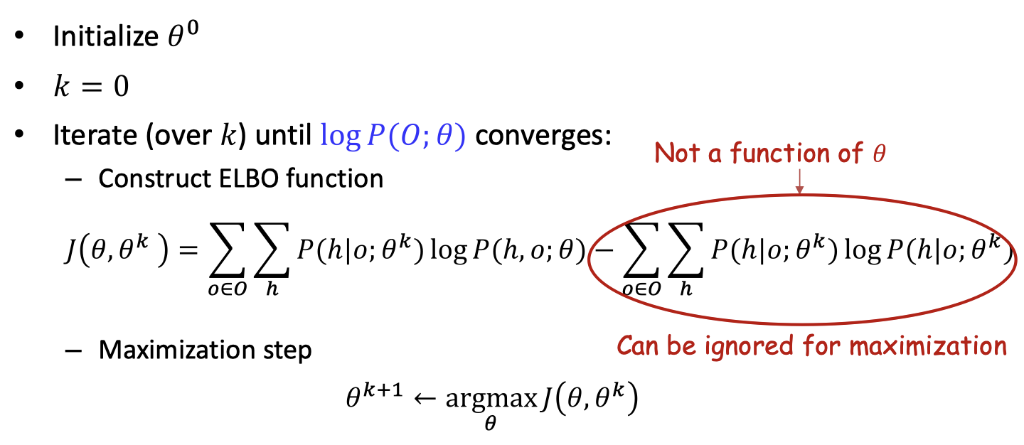
EM algorithm
- Tackle missing data and information problem in model estimation
- Let are observed data
- The logarithm is a concave function, therefore
- Choose a tight lower bound

- Let
- Let

- The algorithm process
EM for missing data
- “Expand” every incomplete vector out into all possibilities
- With proportion (from previous estimate of the model)
- Estimate the statistics from the expanded data

EM for missing information
- Problem : We are not given the actual Gaussian for each observation
- What we want:
- What we have:

- The algorithm process

General EM principle
- “Complete” the data by considering every possible value for missing data/variables
- Reestimate parameters from the “completed” data

Principal Component Analysis

- Find the principal subspace such that when all vectors are approximated as lying on that subspace, the approximation error is minimal
Closed form
- Total projection error for all data
- Minimizing this w.r.t 𝑤 (subject to 𝑤 = unit vector) gives you the Eigenvalue equation
- This can be solved to find the principal subspace
- However, it is not feasible for large matrix (need to find eigenvalue)
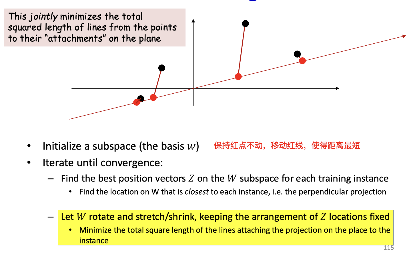
Iterative solution
- Objective: Find a vector (subspace) and a position on such that most closely (in an L2 sense) for the entire (training) data
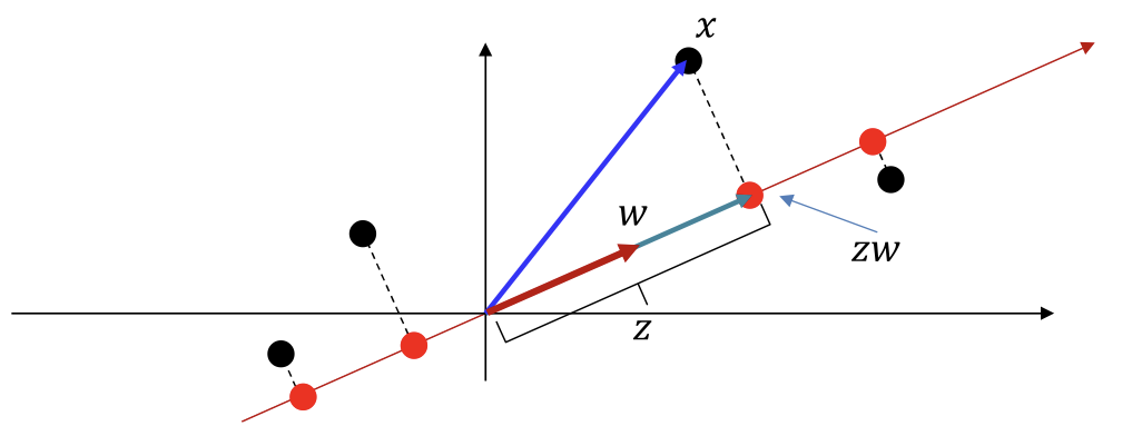
- The algorithm process
PCA & linear autoencoder
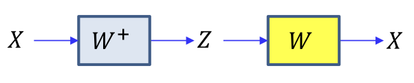
- We put data into the inital subpace, got
- The fix to get a better subpace , etc...
- This is an autoencoder with linear activations !
- Backprop actually works by simultaneously updating (implicitly) and in tiny increments
- PCA is actually a generative model
- The observed data are Gaussian
- Gaussian data lying very close to a principal subspace
- Comprising “clean” Gaussian data on the subspace plus orthogonal noise
