Non-linear extensions of linear Gaussian models.
EM for PCA
- If we knew z for each x, estimating A and D would be simple
x=Az+E
P(x∣z)=N(Az,D)
- Given complete information (x1,z1),(x2,z2)
A,Dargmax(x,z)∑logP(x,z)=A,Dargmax(x,z)∑logP(x∣z)
=A,Dargmax(x,Z)∑log(2π)d∣D∣1exp(−0.5(x−Az)TD−1(x−Az))
- We can get a close form solution: A=XZ+
- But we don't have Z => missing
- Initialize the plane
- Complete the data by computing the appropriate z for the plane
- P(z∣X;A) is a delta, because E is orthogonal to A
- Reestimate the plane using the z
- Iterate
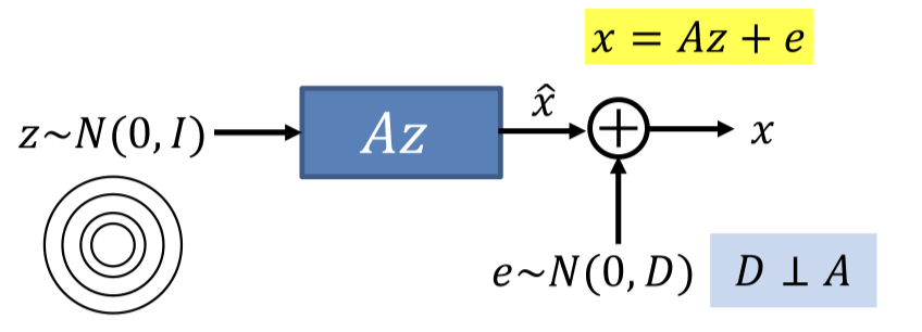
Linear Gaussian Model
- PCA assumes the noise is always orthogonal to the data
- The noise added to the output of the encoder can lie in any direction (uncorrelated)
- We want a generative model: to generate any point
- Take a Gaussian step on the hyperplane
- Add full-rank Gaussian uncorrelated noise that is independent of the position on the hyperplane
- Uncorrelated: diagonal covariance matrix
- Direction of noise is unconstrained
x=Az+e
P(x∣z)=N(Az,D)
- Given complete information X=[x1,x2,…],Z=[z1,z2,…]
A,Dargmax(x,z)∑logP(x,z)=A,Dargmax(x,z)∑logP(x∣z)
=A,Dargmax(x,z)∑log(2π)d∣D∣1exp(−0.5(x−Az)TD−1(x−Az))
=A,Dargmax(x,z)∑−21log∣D∣−0.5(x−Az)TD−1(x−Az)
- We can also get closed form solution
Option 1
- In every possible way proportional to P(z∣x) (Gaussian)
- Compute the solution from the completed data
A,Dargmaxx∑∫−∞∞p(z∣x)(−21log∣D∣−0.5(x−Az)TD−1(x−Az))dz
Option 2
- By drawing samples from P(z∣x)
- Compute the solution from the completed data
The intuition behind Linear Gaussian Model
- z∼N(0,I) => Az
- The linear transform stretches and rotates the K-dimensional input space onto a Kdimensional hyperplane in the data space
- X=Az+E
- Add Gaussian noise to produce points that aren’t necessarily on the plane
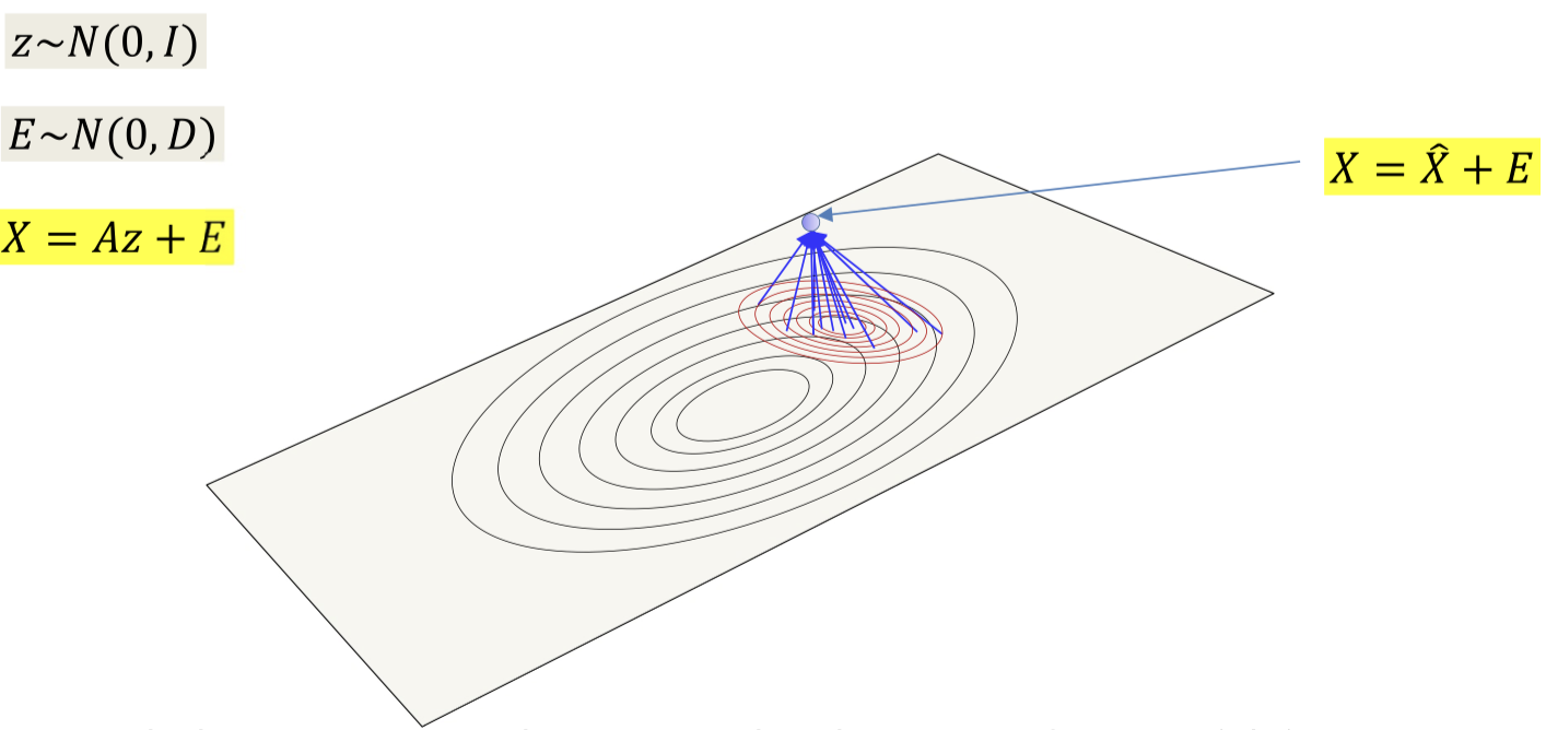
The posterior probability P(z∣x) gives you the location of all the points on the plane that could have generated x and their probabilities
What about data that are not Gaussian distributed close to a plane?
- Linear Gaussian Models fail
- How to do that
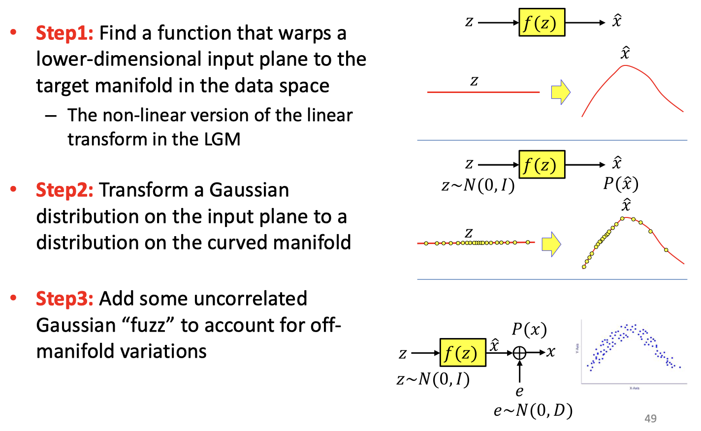
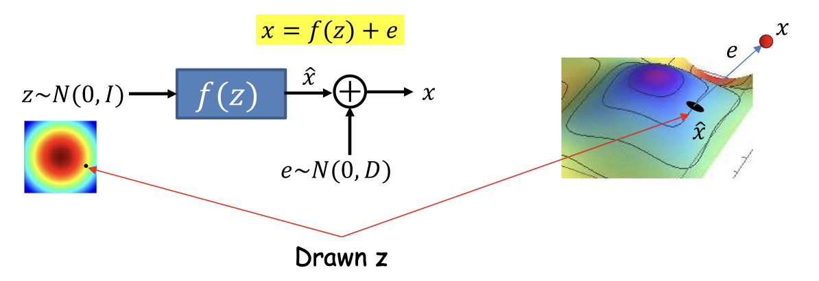
Non-linear Gaussian Model
- f(z) is a non-linear function that produces a curved manifold
- Like the decoder of a non-linear AE
- Generating process
- Draw a sample z from a Uniform Gaussian
- Transform z by f(z)
- This places z on the curved manifold
- Add uncorrelated Gaussian noise to get the final observation
- Key requirement
- Identifying the dimensionality K of the curved manifold
- Having a function that can transform the (linear) K-dimensional input space (space of z ) to the desired K-dimensional manifold in the data space
With complete data
x=f(z;θ)+e
P(x∣z)=N(f(z;θ),D)
- Given complete information X=[x1,x2,…],Z=[z1,z2,…]
θ⋆,D⋆=θ,Dargmax(x,z)∑logP(x,z)=θ,Dargmax(x,z)∑logP(x∣z)
=θ,Dargmax(x,Z)∑log(2π)d∣D∣1exp(−0.5(x−f(z;θ))TD−1(x−f(z;θ)))
=θ,Dargmax(x,Z)∑−21log∣D∣−0.5(x−f(z;θ))TD−1(x−f(z;θ))
- There isn’t a nice closed form solution, but we could learn the parameters using backpropagation
Incomplete data
- The posterior probability is given by
P(z∣x)=P(x)P(x∣z)P(z)
P(x)=∫−∞∞N(x;f(z;θ),D)N(z;0,D)dz
- Can not have a closed form solution

- We approximate P(z∣x) as
P(z∣x)≈Q(z,x)=GaussianN(z;μ(x),Σ(x))
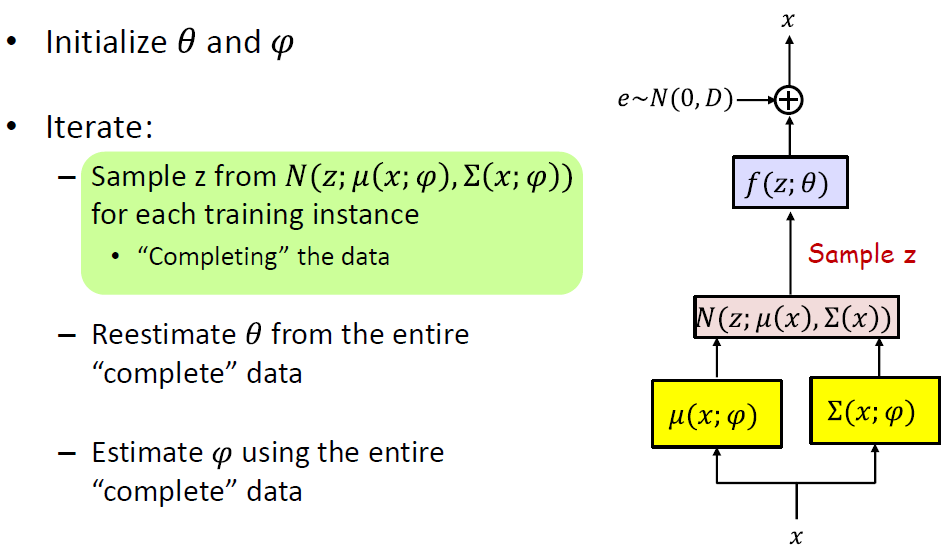
- Sample z from N(z;μ(x;ϕ),σ(x;ϕ)) for each training instance
- Draw K-dimensional vector ε from N(0,I)
- Compute z=μ(x;φ)+Σ(x;φ)0.5ε
- Reestimate θ from the entire “complete” data
L(θ,D)=(x,z)∑log∣D∣+(x−f(z;θ))TD−1(x−f(z;θ))
θ⋆,D⋆=θ,DargminL(θ,D)
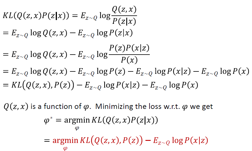
- Estimate φ using the entire “complete” data
- Recall Q(z,x)=N(z;μ(x;φ),Σ(x;φ)) must approximate P(z∣x) as closely as possible
- Define a divergence between Q(z,x) and P(z∣x)
Variational AutoEncoder
- Non-linear extensions of linear Gaussian models
- f(z;θ) is generally modelled by a neural network
- μ(x;φ) and Σ(x;φ) are generally modelled by a common network with two outputs
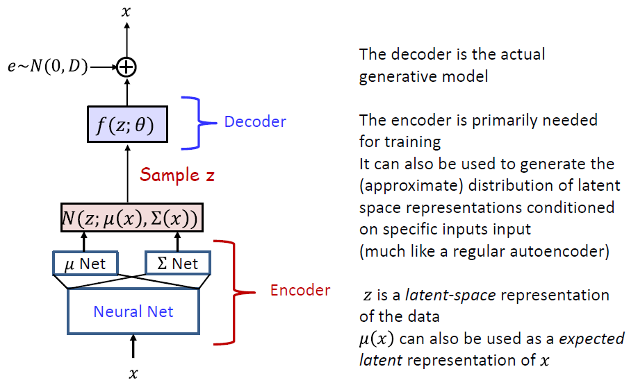
- However, VAE can not be used to compute the likelihoood of data
- P(x;θ) is intractable
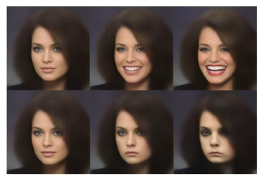
- Latent space
- The latent space z often captures underlying structure in the data x in a smooth manner
- Varying z continuously in different directions can result in plausible variations in the drawn output