Basics of Probability Theory$_{lec1}$

The Calculus of Probabilities

Probability operators

Probability properties

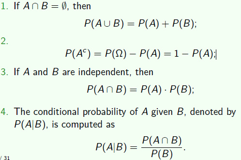
• If $P$ is a probability function, $A$ and $B$ are any two sets in $B$, then
  • $P(\emptyset ) = 0$, where $\emptyset$ is the empty set
  • $P(A) \le 1$
  • $P(B \cap A^c ) = P(B) - P(A \cap B)$
  • $P(A \cup B) = P(A) + P(B) - P(A \cap B)$
  • If $A \subset B$, then $P(A) \le P(B)$
• Events $A_1$ and $A_2$ are pair-wise independent (statistically independent) if and only if
  • $P(A_1 \cap A_2) = P(A_1)P(A_2)$
• mutually independent:
  • $P(A_1 \cap A_2 \cap ... \cap A_n) = P(A_1)P(A_2)...P(A_n)$
• Note the difference between independent and mutually exclusive
  • mutually exclusive: $cov(X,Y) = 0$
  • independent: $P(X,Y) = P(X)P(Y)$
• Let $A$and$B$ be events with $P(B) > 0$. The conditional probability of A given$B$, denoted by $P(A|B)$, is defined as
  • $P(A|B) = \frac{P(A\cap B)}{P(B)}$
• Total probability theorem:
  • $P(A) = P(B_1) P(A|B_1) + P(B_2) P(A|B_2) + P(B_3) P(A|B_3)$
  • $P(A) = \sum\limits_{i=1}^{n}P(B_i) {(A|B_i)}$
• Bayes' Theorem
  • $P(B_i|A) = \frac{P(A|B_i)P(B_i)}{\sum\limits_{k=1}^{n}P(A|B_k)P(B_k)}$

Counting

• inclusion-exclusion
  • $|A\cup B| = |A| + |B| - |A\cap B|$
• Permutations and combinations
  • $P(n,m) = \frac{n!}{(n-m)!}$
  • $C(n,m) = \frac{n!}{m!(n-m)!}$

Random Variable$_{lec2}$

• A random variable (r.v.) X is a function from sample space of an experiment to the set of real numbers in R:
  • $\forall w\in \Omega, X(w) = x \in R$
• Note that a random variable is a function, and not a variable, and not random.

Cumulative distribution function

• The cdf of a r.v denoted by $F_x(X)$ is defined by :
  • $F_X(x) = P_X(X\le x)$
• $\lim _{x \rightarrow -\infty} = 0$
• $\lim _{x \rightarrow \infty} = 1$
• $F(x)$ is nondecreasing function of $x$
• $F(x)$ is right-continuous
• two r.v.s that are identically distributed are not necessarily equal.

Probability mass function

• The pmf of a discrete r.v. $X$ is given by $f_X(x) = P(X = x)$

Probability density function

• The probability density function or pdf, $f_X(x)$, of a continuous r.v. $X$ is the function that satisfies:
  • $F_X(x) = \int_{- \infty}^x f_X(t) dt$
• $X$ has a distribution given by $F_X (x)$ is abbreviated symbolically by $X \sim F_X (x)$ or $X \sim f_X (x)$.

Joint distribution$_{lec3}$

• $P((X,Y)\in A) = \sum_{(x,y)\in A} f(x,y)$
• $P((X,Y)\in A) = \int \int_A f(x,y)dxdy$
• $f_X(x) = \int_{-\infty}^{+\infty}f_{X,Y}(x,y)dy$
• $\frac{\partial ^2F(x,y)}{\partial x\partial y} = f(x,y)$
• $f(x|y) = \frac{f(x,y)}{f_Y(y)}$
• if $f(x,y) = f_X(x)f_Y(y)$, then $X,Y$ are independent.
  • 若变量可分离，则不需要计算边际分布，直接可判断相互独立

Bivariate function

• $(X,Y)$ be a bivariate r.v, consider a new bivariate r.v $(U,V)$, define by $U = g_1(X,Y)$ and $V = g_2(X,Y)$

Transformation of discrete

• $B = \{(u,v) | u = g_1(x,y), v=g_2(x,y) ,(x,y) \in A \}$
• $A_{uv} = \{ (x,y)\in A | u = g_1(x,y), v=g_2(x,y) \}$
• $f_{u,v} = P(I = u,V= v) = P((X,Y) \in A_{uv}) = \sum_{(x,y)\in A_{uv} } f_{X,Y}(x,y)$

Transformation of continuous

$J=\left|\begin{array}{ll} \frac{\partial x}{\partial u} & \frac{\partial x}{\partial v} \\ \frac{\partial y}{\partial u} & \frac{\partial y}{\partial v} \end{array}\right|$

• $f_{u,v} = f_{X,Y}(h_1(u,v),h_2(u,v))|J|$
• 这是用反函数求解的方法，若有些题无法用反函数求解，则使用累计密度函数带入计算

Expectation & covariance$_{lec4}$

Expectation value

• denoted as $R(g(X))$:

$\begin{aligned} &E(g(X))=\int_{-\infty}^{+\infty} g(x) f_{X}(x) \text { if } X \text { is continuous }\\ &=\sum_{x \in X} g(x) P(X=x) \text { if } \mathrm{X} \text { is discrete } \end{aligned}$

• note: expectation is not always exist
  • Cauchy r.v, the pdf:
    • $f_X(x) = \frac{1}{\pi (1+x^2)}$
  • $E(X) = \infty$

Linearity of expectations

• $E(ag_1(X) + bg_2(X) + c ) = aE(g_1(X)) + bE(g_2(X)) + c$
• if $a \le g_1(x) \le b$ for all $x$, then $a\le E(g_1(X)) \le b$

Uniform exponential relationship

• can use uniform distribution to form other distribution: exponential, normalization, which is actually do in computer
• suppose $X \sim U(0,1)$,let $Y = g(X) = -\log X$
  • $F_Y(y) = P(Y\le y) = P(-\log X \le y) = P_X(x\ge e^{-y}) = 1- e^{-y}$
  • $f_Y(y) = e^{-y}$
  • so $Y \sim \exp(1)$

Moment

• For each integer $n$, the $n-th$ moment of $X$, is $\mu_n = E(X^n)$
• The $n-th$ central moment of $X$, $\mu_n = E(X - \mu)^n$

Variance

• The variance of a r.v. $X$ is its second central moment:

  • $var (X) = E(X-\mu)^2$

• $var(X) = E(X^2) - (E(X))^2$

Nonlinearity of variance

• $var(aX+b) = a^2var(X)$
• if $X$ and $Y$ are tow independent r.v.s on a sample space $\Omega$, then:
  • $var(X+Y) = var(X) + var(Y)$

Independence

• if $X$ and $Y$ are independent r.v.s on a sample space $\Omega$, then:
  • $E(XY) = E(X)E(Y)$
  • $var(X+Y)= var(X)+var(Y)$
  • $var(X-Y) = var(X) +var(Y)$

Moment Generating Function

• can be used to calculate moment
• the moment generating function of $X$, denoted by $M_X(t)$, is:
  • $M_X(t) = E(e^{tX})$
• $M_{aX+b}(t) =e^{bt}E_X(at)$
• is applied to Chernoff bound
• if the expectation dose not exist, the moment generating function dose not exist.
• $X$ is continuous, $M_X(t) = \int _{-\infty}^{+\infty} e^{tx}f_X(x) dx$
• $X$ is discrete, $M_X(t) = \sum_xe^{tx}P(X= x)$

Theorem

• if $X$ has moment generating function $M_X(t)$, then :
  • $E(X^n) = M_n^{(n)}(0)$
• where we define:
  • $M_X^{(n)}(0) = \frac{d^n}{dt^n} M_X(t) | _{t=0}$
• can be used to calculate Gamma $E(X)$

Property

• $M_{aX+b}(t) = e^{bt}M_X(at)$

Covariance

• The covariance and correlation of $X$ and $Y$ are the numbers defined by:
  • $Cov(X,Y) = E((X-\mu _X)(Y-\mu_Y))$
  • $\rho_{XY} = \frac{Cov(X,Y)}{\sigma_X\sigma_Y}$
• $Cov(X,Y) = E(XY) - \mu_X\mu_Y$
• if $X,Y$ are independent r.v.s, then $Cov(X,Y) = 0$ and $\rho_{XY} = 0$
• $Var(aX+bY) = a^2Var(X) + b^2Var(Y) + 2abCov(X,Y)$
• 相关系数只能说明是否存在线性关系，若等于0，不能说没有关系。
  • 但若使用$\rho(X^2,Y)$，也可以衡量。
  • 由于任何函数都可以用多项式拟合，因此都可以用相关系数衡量

Bivariate normal pdf

• $f(x,y) = (2\pi \rho_X\rho_Y\sqrt{1-\rho^2})^{-1}\cdot \exp(-\frac{1}{2(1-\rho^2)}((\frac{x-\mu_x}{\sigma_X})^2 - 2\rho(\frac{x-\mu_x}{\rho_X})(\frac{y-\mu_Y}{\rho_Y}) + (\frac{y-\mu_Y}{\sigma_Y})^2))$
• marginal distribution
  • $X\sim N(\mu_X,\sigma_X^2)$
  • $Y\sim N(\mu_Y,\sigma_Y^2)$
• $\rho = \rho_{XY}$
• $aX+bY \sim N(a\mu_X+b\mu_Y,a^2\sigma_X^2 + b^2\sigma_Y^2 + 2ab\rho \sigma_X\sigma_Y)$

conditional expectation$_{lec4}$

Theorem

• $E(X) = E(E(X|Y))$
  • 可以理解为先分组求期望，与直接求期望一样
• $Var(X) = E(Var(X|Y)) + Var(E(X|Y))$
  • 可以理解为组内方差的期望 + 组间方差

Mixture distribution

Binomial-Poisson hierarchy

• if $X| Y \sim Binomial(Y,P),Y\sim Possion(\lambda)$:
• $P(X=x)= \sum P(X=x,Y=y) = \sum P(X=x|Y=y)P(Y=y) = \frac{(\lambda P)^x}{x!} e^{\lambda P}$
• $\therefore X\sim Possion(\lambda P)$
• using $E(X) = E(E(X|Y))$, can easily get $E(X) = E(pY) = p\lambda$

Beta-binomial hierarchy

• if $X|P \sim Binomial(n,p),P\sim \beta (\alpha,\beta)$

• so $E(X) = E(E(X|P)) = E(np) = \frac{n\alpha}{\alpha + \beta}$